One of the many simplifying hypotheses that was made in developing the preliminary epidemiological model in the previous chapter concerns the number of sites, which was kept constant for the entire duration of epidemics. The implicit assumption was therefore made that a fixed initial stock of healthy sites was set at the beginning of an epidemic (and of a crop cycle), and left to decline under the effect of the rate of infection as an epidemic progresses. A crop that does not grow for 100 days does not exist. In this chapter, we want to account for crop growth, that is to say, the progressive build-up of healthy sites. Furthermore, we wish to account for the fact that, as time goes by, many sites senesce, implying that, as the crop grows and the epidemic builds up, fewer sites are made available to infection, not only because they might become infected (and so, not available anymore to infection), but also simply because they are senesced. Lastly, we would like to achieve these goals with as few, simple, hypotheses as possible.
Adding components (and hypotheses) to the model
Let us use the model developed in the previous chapter to incorporate crop growth and senescence. The overall structure of the modified model is shown in Fig. 5.1.
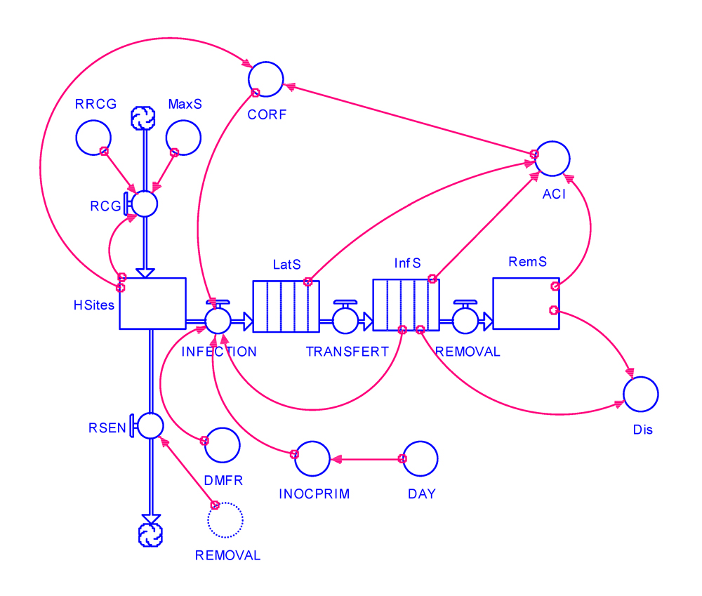
Figure 5.1. One needs to model crop growth, and thus create a rate of crop growth (RCG). For the sake of simplicity, let us assume that crop (site) growth is logistic. We thus have to create a carrying capacity, which represents the maximum size the site population may achieve, MaxS.
As for all the site-variables (most of which are state variables in the model), the dimension of the parameter MaxS is [Nsite], although the considered system has a finite size (e.g., 1 m2 of a wheat crop in a large field). The proper dimension of site variables thus should be [Nsite.L-2]. However, from the onset of the previous chapter, the size of the system - again, an important hypothesis the model has - has been implicit. Thus, we shall retain [Nsite] as a dimension from now on.
The logistic rate of growth is proportional to the amounts of individuals (i.e., sites) that are contributing to growth. Let us further assume that only healthy sites (HSites) do so, that is to say that, once infected (latent, infectious, or removed), infected sites no longer contribute to growth. The rate of crop growth can therefore be written as:
RCG = RRCG * HSites * (1-(HSites/MaxS))
Let us also assume that crop growth starts with a small number of sites, 100, with a carrying capacity of 100,000 sites (MaxS = 100,000), and a relative rate of growth of 0.1 site·site-1·day-1. This latter assumption implies that each site gives birth to 0.1 new site at each time step. The result of crop (site) growth in the absence of disease is shown in Fig. 5.2.

Figure 5.2. Simulated crop growth (number of sites, blue) and of crop growth rate (red) in a healthy crop. Horizontal axis: time (days); vertical axis: numbers of sites.
We want next to incorporate senescence in the model. Senescence is indeed a very complex process (e.g., Gardener et al., 1985; Lim et al., 2003), which occurs in any crop stand, whether healthy or diseased. To incorporate such processes is tempting. Doing so would however imply involving complicated processes, and we would rather keep the model as simple and tractable as possible. A comparatively simple approach would at least involve including
development, that is, the successive transition of sites through different physiological stages, in addition to
growth, that is, in addition to the mere incrementing (and/or subtraction) of sites over time. Crop development will be addressed in the following chapters. What is proposed here is to take a shortcut, and assume that the rate of senescence (RSEN) is numerically equal to the rate of removal from the epidemiological process:
RSEN = REMOVAL
While another hypothesis will be discussed at the end of this chapter, let us ponder now what this equation implies. As the crop is being established, very little disease, if any (see below), is present. At that stage, one can safely assume that both removal and senescence are equal and null. In a second stage, once infected, sites go through the delays of latency and infectiousness. This takes a few days, corresponding to the latency period
p then the infectious period
i. During this second stage, removal is at most small, and so is senescence. In a third stage, as the epidemic truly builds up, post-infectious sites start to accumulate as removed sites. In this third stage, senescence, too, tends to increase. Thus, for any disease, one may assume that equating the rates of senescence to that of removal is phenomenologically acceptable (they coincide over time), although this reasoning is not physiologically or epidemiologically correct; senescence occurs in absence of disease, in the same way as disease may not necessarily lead to senescence. If we take as an example a necrotrophic pathogen infecting the foliage, the assumption however appears appropriate; removed sites often senesce much faster. Then again, this is generally not the case in biotrophic pathogens, as with many leaf rusts on mono- or dicots. Let us accept this as a working hypothesis for the time being.
A third change has to do with the initiation of epidemics. In the preliminary model of the previous chapter, epidemics started off with an influx of 100 infections as soon as the process started. Since we now start off with 100 (healthy) sites, having them all infected at such an early stage of crop growth will not do; crop growth would stop immediately and such a thing is not realistic. Instead, the epidemic is started later on.
In order to do so, we write INOCPRIM as:
IF (DAY=20) THEN 100 ELSE 0
instead of:
IF (DAY=1) THEN 100 ELSE 0
which was used in the model of Chapter 4. Furthermore, all the other parameters are set to the same default values as in Chapter 4.
Instead of changing the original structure of epidemic onset we now assume that 100 infections take place 20 days after crop growth has started. The listing of the program is given in Appendix 5.1 at the end of this chapter.
Verifying the model: model behavior
A first question is whether such changes have affected the model behavior: not only have crop growth and senescence been included, but the onset of disease has been delayed by 20 days. These are important changes that need to be addressed first.
Let us first compare the outputs of the model of Chapter 4 and those of the new model of Fig. 5.1, both of them simulating epidemics with onset times at t = 20 days.
Fig. 5.3 shows dramatic differences in outputs. One is that, in the outputs of the new version of the model (Fig. 5.3b), we do not observe a steady decline of healthy sites over time. The new outputs show an initial increase then a decline. The maximum number of healthy sites is also strongly reduced. Other differences concern the diseased sites. Overall, the number of diseased sites is reduced when crop growth is taken into account. In the former (no crop growth, Fig 5.3a) simulation, one sees a sigmoid pattern followed by a decline of the latent sites. The new outputs show a regular increase of the infectious, removed, and accumulated diseased sites over time, while the progress curve for latent sites is sigmoid. These differences in behavior in the dynamics of the disease state variables are caused by the comparatively smaller amount of sites that are available (healthy) at the early stage of the epidemic, and which only increase progressively over time. Thus, at each time step over time, the amount of healthy sites, i.e. the carrying capacity of the disease to develop, varies: it initially increases at a moderate rate (because crop growth being logistic is proportional to a relatively small number of healthy sites), and then the carrying capacity tends to progressively decrease as disease intensifies. In simple words, one could say that the disease has less room to develop.
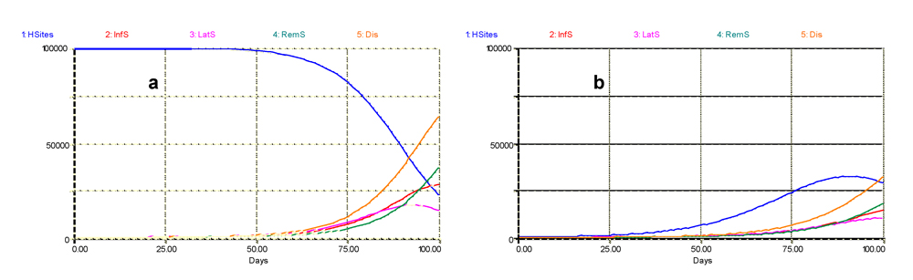
Figure 5.3. Simulated dynamics of sites (healthy, infectious, latent, removed, and total diseased) in a crop where growth and senescence are not (a, left) or are (b, right) simulated. Horizontal axis: time (days); vertical axis: numbers of sites.
Effect of varying rates of crop growth
One important change in the initial model is therefore crop growth. We can conduct a sensitivity analysis, where the relative (or intrinsic) rate of growth is changed. Fig. 5.4 shows the outcomes, in terms only of healthy and diseased sites. With RRCG = 0.05, both crop growth and disease progress are negligible: this is because healthy sites are infected as soon as they are produced, preventing further growth (to which only healthy sites can contribute) occurring. With RRCG = 0.09, some crop growth occurs, but diseased sites follow a regularly increasing curve, ending, in relative terms, with high disease intensity (i.e., Dis/(Dis+HSites), of roughly 70%. With RRCG = 0.10 (which is the reference value in the earlier verifications), crop growth follows a sigmoid pattern, and diseased sites build up regularly, reaching, in relative terms, a fraction of disease lower than in the previous run. Thus at the end of the epidemic, intensity is about 50%. Interestingly, this relative expression of terminal disease intensity is the same in the following runs. With RRCG = 0.11 or 0.15, crop growth becomes faster, and shows a definite terminal decline. This decline is caused by the corresponding increase of disease, which now rapidly has a larger carrying capacity as the dynamics of growth unfolds. When RRCG = 0.20, crop growth reaches the maximum site carrying capacity (100,000 sites), but collapses as disease increases exponentially at a high rate: the accumulation of healthy sites provides 'room for maneuver' for disease increasing almost freely.

Figure 5.4. Simulated epidemics at varying relative rates of crop growth, RRCG. Graphs are showing only the simulated numbers of healthy and diseased sites. RRCG values are given in each graph. Horizontal axis: time (days); vertical axis: numbers of sites.
Effect of the daily multiplication factor, DMFR
The previous chapter addressed a series of epidemiological parameters in their effects on the behavior of the model. Let us look at one of them, the daily multiplication factor (DMFR) of an infectious lesion. Three values for DMFR are tested in Fig. 5.5: DMFR = 0.30, which is the standard value used in this chapter, and DMFR = 0.25 or DMFR = 0.35.
With DMFR = 0.25, crop (site) growth follows a simple sigmoid pattern. Latent, infectious, and removed, as well as visibly diseased (infectious + removed) sites increase exponentially, hampering crop growth, but only to a marginal extent. By contrast, when DMFR is increased to a value of 0.35, crop growth is strongly suppressed, and the number of healthy sites shows a clear decline at the end of the run. A similar decline also occurs for the latent and infectious sites, leading to a tapering-off of the visibly diseased sites.
These three runs also indicate that, with increased DMFR values, the terminal relative disease intensities, if expressed in absolute terms (i.e., [Nsite]), do not vary very much. However, if expressed in relative terms (i.e., %, that is [Nsite.Nsite-1]), a very strong decline is apparent. This additional set of runs thus underline the very strong difference in interpretation attached in expressing disease in absolute (that is, numbers, as the state variables used here) or in relative terms, which is so common in the epidemiological literature, where many results are reported as percentages.
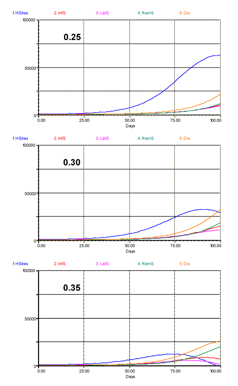
Figure 5.5. Simulated epidemics at varying values of DMFR: 0.25, 0.30, and 0.35. Graphs are showing the variation of healthy, latent, infectious, removed sites, and the total number of (visibly) diseased sites. 1: healthy sites; 2: infectious sites; 3: latent sites; 4: sites removed from the epidemiological process; 5: visibly diseased (infectious and removed) sites. Horizontal axis: time (days); vertical axis: numbers of sites.
Modeling senescence in a different manner
One of the hypotheses the model discussed so far implies that the rate of senescence is equal to the rate of removal of diseased sites. Even though explanations were given to support this hypothesis, at least from a phenomenological standpoint, further analysis is useful.
One could, for instance, assume that senescence of healthy sites is only related to plant physiology, and could be expressed by an intrinsic rate of ageing of healthy tissues or a rate of removal of healthy sites (RRemHS). One could also assume that senescence is influenced by both disease and ageing. One simple assumption in that case is to consider the two processes additive, that is, without interaction, and write:
RSEN = RRemHS*HSites + RRemDS*REMOVAL
where RRemDS is an intrinsic rate of removal of healthy sites caused by disease.
The above equation was incorporated in the model and the following parameter values: RRemHS = 0.00001 and RRemDS = 0. 0001 were used. These values are very small, because they are relative rates affecting processes that take place late in the growing season and the epidemic, and because the value for RRemDS, which actually is a modifier of a rate, is 10 times larger than the value of RRemHS (the rate of removal of diseased sites, Fig. 5.1). The outputs are shown in Fig. 5.6, and can be compared with the right hand-side of Fig. 5.3. Both graphs show much similarity, except for the decline of healthy sites at the end of the epidemic, which is more visible in Fig. 5.2. This is logical, since senescence is only caused by disease in this case. It thus seems that the earlier hypothesis made in the development of the model is acceptable.

Figure 5.6. Simulated outputs with senescence of healthy tissues made dependent on both physiology and plant disease. 1: healthy sites; 2: infectious sites; 3: latent sites; 4: sites removed from the epidemiological process; 5: visibly diseased (infectious and removed) sites. Horizontal axis: time (days); vertical axis: numbers of sites.
Revisiting hypotheses
As in the previous chapter, the model used here implies a number of assumptions, some of which are explicit, and others, implicit. Let us address two explicit assumptions.
A first hypothesis is that crop (site) growth is logistic. In many cases, this assumption is not appropriate. This is especially the case if the sites under consideration were root-sites: root growth, in many crops, is very rapid in the beginning of the growing season, and stops long before the reproductive stage (in annual crops) is over (e.g., Gardner et al., 1985). The aerial tissues of a crop canopy also have an asymmetric rate of growth, which rapidly increases in the beginning of the growing season, and progressively decreases later. As a result, a flush of healthy sites would become rapidly available to possible infection, with strong differences in the shape of disease progress. There are a number of equations to account for such asymmetrical growth, for the host or for the pathogen (e.g., Kranz, J., 1976; 1990; Berger, 1981; Madden et al., 2007), and we leave it to the interested reader to try and incorporate them in the model, to see the epidemiological outcomes.
The second, actually very strong, hypothesis is that we assumed that only healthy sites (HSites) contribute to crop growth. This hypothesis can in turn be partitioned into two questions: (1) are all diseased sites truly not contributing to crop growth, and (2) are all healthy sites equally contributing to crop growth, creating a differential in disease occurring in some healthy sites rather than others.
The first question may, to some extent, be related to the biology of the considered pathogen. If one is dealing with a necrotroph (Cooke and Whipps, 1980), then infected sites become very rapidly dysfunctional (e.g., Savary et al., 1990; Bastiaans, 1993; Lopes and Berger, 2001), and the underlying hypothesis seems to hold. If one is dealing with a biotroph (e.g., Ayres, 1981; Mendgen, 1981), then infected sites still continue to be functional, but their photosynthetic activity is only directed to the maintenance, growth, and reproduction of the pathogen (e.g., Savary et al., 1990; Lopes and Berger, 2001). In the case of some host-pathogen interactions, the biotrophic pathogen in fact enhances the photosynthetic activity of infected tissues (e.g., Ayres, 1981). Thus, one may consider a possible under-estimate of the effect of infection on the population of sites, at least among the infected ones, and possibly, among the healthy sites. The latter remark brings us back again to the underlying hypothesis of evenly distributed disease in plant tissues, in this case, in terms of crop growth – disease progress relationships. This topic will be further addressed in the next chapters. There are "shades of grey" in the trophic relationships between plants and their pathogens, since a great number of plant pathogens stand between the two extremes – biotroph vs. necrotroph.
The relationships between crop growth and epidemiological dynamics are, indeed, complex. The model structure presented here is a very simple one, to which many details would have to be added in order to address a specific pathosystem in any detail. The phrase "shades of grey" will return in the next chapter, in a completely different setting.
Perspectives
This chapter introduces in a very simple manner the complex linkages between a growing crop and the epidemic of a disease. Much has been written on the topic, which forms a strong component of disease management. The questions of relationships between the host and the pathogen, and between crop growth and disease (and harmful agents, in general) will be addressed further in the next chapters.
Simulations
The STELLA® model provided with this chapter (EPIDEMGRO.STMX) will allow you to explore the model structure and equations, and run the model with varying values of the intrinsic rate of crop growth, RRCG and DMFR, to see the effects of such changes on the simulated epidemics.
Summary
- Incorporating crop growth in a simulation model completely alters the course of an epidemic, whose shape becomes, overall, more realistic.
- Overall, crop growth provides room for maneuver for the course of epidemics, which depends on the dynamics of the available carrying capacity of the host population.
- The rate of crop growth itself has also a very strong effect on the modeled dynamics of epidemics and their outcomes.
- Many hypotheses might be implemented to model crop growth and senescence; in this section, these hypotheses were kept as simple as possible and the underlying assumptions are discussed.
- There can be very large implications in expressing disease intensity as an absolute amount of disease vs. as a fraction of host tissues, that is, disease percentage.
- A STELLA® model (EPIDEMGRO.STMX) allows you to explore the model behavior with varying values of the intrinsic rate of crop growth, RRCG and DMFR.
References
Ayres, P.G. 1981. Powdery mildew stimulates photosynthesis in uninfected leaves of pea plants. Phytopathologische Zeitschrift 88: 312-318.
Bastiaans L. 1993. Effects of leaf blast on growth and production of a rice crop. 1. Determining the mechanism of yield reduction. Netherlands Journal of Plant Pathology 99:323-334.
Berger, R.D. 1981. Comparison of the Gompertz and logistic equations to describe plant disease progress. Phytopathology 71:716-719.
Gardner, F.P., Pearce, R.B., and Mitchell, R.L. 1985. Physiology of Crop Plants. Iowa University Press, Ames.
Cooke, R.C., and Whipps, J.M. 1980. The evolution of modes of nutrition in fungi parasitic on terrestrial plants. Biological Reviews 55:341-360.
Kranz, J., 1976. Effect of some plant diseases on the loss of leaves. Zeitschrift fur Pflanzenkrankheiten und Pflanzenschutz 72:1373-1377.
Kranz, J. (Ed.) 1990. Epidemics, their Mathematical Analysis and Modeling: an introduction. Pages 1-11 in: Epidemics of Plant Diseases. Second Edition, Springer Verlag, Berlin.
Lim, P. O., Woo H. R., and Nam H. G. 2003.Molecular genetics of leaf senescence in Arabidopsis. Trends in Plant Science 8:272-278.
Lopes, D.B., and Berger, R.D., 2001. The effects of rust and anthracnose on the photosynthesis competence of diseased bean leaves. Phytopathology 91:212-220.
Madden, L.V., Hughes, G., and Van den Bosch, F. 2007. The Study of Plant Disease Epidemics. The American Phytopathology Press. St Paul, Minnesota, USA.
Mendgen, K. 1981. Nutrient uptake in rust fungi. Phytopathology 71:963-964.
Robert, C., Bancal, M.O., and Lannou, C. 2002. Wheat leaf rust uredospore production and carbon and nitrogen export in relation to lesion size and density. Phytopathology 92:762-768.
Savary, S., De Jong, P.D., Rabbinge, R., and Zadoks, J.C. 1990. Dynamic simulation of groundnut rust, a preliminary model. Agricultural Systems 32:113-141.
Suggested reading
Berger, R.D. 1977. Application of epidemiological principles to achieve plant disease control. Annual Review of Phytopathology 15:165-183.
Jeger, M.J. 1986. Asymptotic behaviour and threshold criteria in model plant disease epidemics. Plant Pathology 35:355-361.
Jeger, M.J., and Van Den Bosch, F., 1994. Threshold criteria for model plant disease epidemics. I. Asymptotic results. Phytopathology 84:24-27.
Jeger, M.J. 2004. Analysis of disease progress as a basis for evaluating disease management practices. Annual Review of Phytopathology 42:61-82.
Zadoks, J.C., and Schein, R.D. 1979. Epidemiology and Plant Disease Management. Oxford University Press, New York.
Zadoks, J.C., and Rabbinge, R., 1985. Modelling to a purpose. Pages 231-244 In: Advances in Plant Pathology. Vol. 3. Mathematical Modelling of Crop Diseases. C.A. Gilligan, ed. Academic Press, London.
Exercises and questions
Questions
1. The rate of crop growth with the hypothesis of carrying capacity can be written as
a. RCG = RRCG*HSites
b. RCG = RRCG*MaxS*(1-(HSites/MaxS))
c. RCG = RRCG*HSites*(1+(HSites/MaxS))
d. RCG = RRCG*HSites*(1-(HSites/MaxS))
2. The dimension of the relative rate of crop growth, RRCG is
a. [N]
b. [N.T-1]
c. [N.N-1.T-1]
d. [N.T-2]
3. An increase in the rate of crop growth will
a. increase the rate of infection
d. decrease the rate of infection
c. not affect the rate of infection
Answers to questions
1. d: RCG = RRCG*HSites*(1-(HSites/MaxS))
2. c: [N.N-1.T-1]
3. a: increase the rate of infection
Appendix 5.1. Program listing of EPIDEMGRO
HSites(t) = HSites(t - dt) + (RCG - INFECTION - RSEN) * dt
INIT HSites = 100
INFLOWS:
RCG = RRCG*HSites*(1-(HSites/MaxS))
OUTFLOWS:
INFECTION = (DMFR*CORF*InfS)+INOCPRIM
RSEN = REMOVAL
InfS(t) = InfS(t - dt) + (TRANSFERT - REMOVAL) * dt
INIT InfS = 0,0,0,0,0,0,0,0,0,0
TRANSIT TIME = 10
INFLOW LIMIT = INF
CAPACITY = INF
INFLOWS:
TRANSFERT = CONVEYOR OUTFLOW
OUTFLOWS:
REMOVAL = CONVEYOR OUTFLOW
LatS(t) = LatS(t - dt) + (INFECTION - TRANSFERT) * dt
INIT LatS = 0,0,0,0,0,0
TRANSIT TIME = 6
INFLOW LIMIT = INF
CAPACITY = INF
INFLOWS:
INFECTION = (DMFR*CORF*InfS)+INOCPRIM
OUTFLOWS:
TRANSFERT = CONVEYOR OUTFLOW
RemS(t) = RemS(t - dt) + (REMOVAL) * dt
INIT RemS = 0
INFLOWS:
REMOVAL = CONVEYOR OUTFLOW
ACI = LatS+InfS+RemS
CORF = 1-(ACI/(ACI+HSites))
DAY = TIME
Dis = InfS+RemS
DMFR = 0.3
INOCPRIM = IF (DAY=20) THEN 100 ELSE 0
MaxS = 100000
RRCG = 0.1

