Modeling the effects of injuries caused by pests (diseases, insects, and weeds) on crop growth and yield requires, as a first stage, the modeling of growth and yield of a crop in absence of injuries. This chapter will take you through the main processes involved in crop growth, how these processes are represented in a quantitative and dynamic manner, and how they are implemented into a simple model, which you can explore and run. This chapter starts with the RI-RUE paradigm, which has strong connections with the modeling of yield losses, and provides a very simple and robust framework to address crop growth under a set of biophysical constraints.
The RI-RUE concept
RI is the radiation intercepted by the crop canopy and can be written in a simple way using Beer's law (Monsi and Saeki, 1953, see also, Goudriaan and van Laar, 1994; Whisler et al., 1986; Thornley and France, 2007) as:
 | (7.1) |
where
RAD is the global solar radiation, that is, the incident radiation above the canopy;
k is the extinction coefficient; and
LAI is the Leaf Area Index (i.e., the area of leaf per area of ground soil, dimension = [L2.L-2] with units m2·m-2). The parameter
k depends on the direction of the radiation and on the orientation of the leaves. Average values for canopies with erect and horizontal leaves are about 0.6 and 0.8, respectively (Penning de Vries et al., 1989). The intercepted radiation increases with LAI, but the rate of increase diminishes as LAI increases. For a given value of LAI, the intercepted radiation is larger for canopies with horizontal than erect leaves (Fig. 7.1).
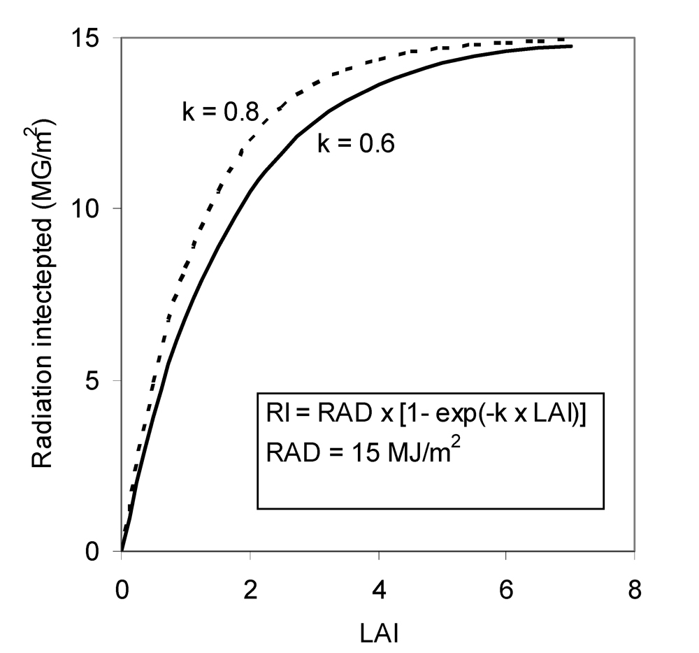
Figure 7.1.
Relationships between radiation intercepted and LAI.
Monteith (1977) established a robust, linear relationship between the accumulated crop biomass and
RI. He introduced the concept of Radiation Use Efficiency (RUE), which can empirically be estimated as the slope value from the linear regression of accumulated biomass over accumulated
RI.
RUE represents the conversion of radiation energy into biomass. In other words,
RUE represents the amount of dry biomass (DBM) produced per unit of radiation energy intercepted by the crop canopy. An
RUE value for crops under non-limiting conditions is about 1.4 g·MJ-1, or approximately 2.8-3.2 g·MJ-1 of photosynthetically active radiation (PAR; Monteith, 1977). Using Monteith's framework, the accumulated dry biomass over a time interval [0, t], (DBMt) can therefore be written as:
 | (7.2) |
This framework establishing relationships between crop growth, radiation interception, and
RUE has been used in a very wide range of examples to model crop growth in a simple way (e.g., Johnson et al., 1986; Sinclair, 1986; Steer et al., 1993; Richter et al., 2001; Kiniri et al., 2004). This framework is used here because it has also enabled addressing the effects of harmful organisms on crop growth in a generic, synthetic manner (see Chapter 8).
Main processes involved in crop growth captured into a simple crop growth simulation model for attainable growth and yield – GENECROP
Model system and structure
The time step of the GENECROP model is one day, and the system modeled is 1 m2 of crop. The different processes determining crop growth are embedded into the model in three components, which deal with: (1) the dynamics of crop development, (2) the accumulation of crop biomass, and (3) the growth in numbers of tillers (or shoots). A complete listing of the program can be found in Appendix 7.1.
The model structure can be explored by opening the STELLA model GENECROP.STMX and clicking on the "explore model" button. The model equations can be viewed by selecting the "equation" level on the left part of the panel when opening the file. The flowchart of the model is given in Fig. 7.2.
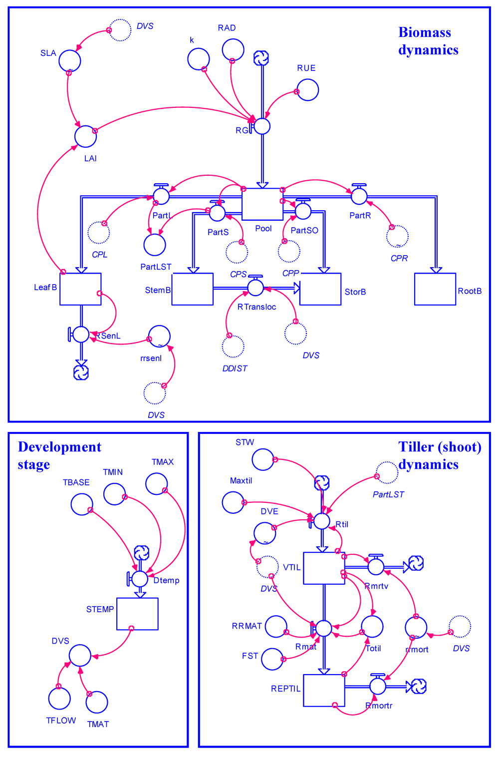
Figure 7.2. Flowchart of GENECROP, a generic model for attainable crop growth.
The main processes involved over the course of a crop cycle are: photosynthesis, biomass partitioning in growing plants, leaf senescence, and yield build-up. Most of these processes are driven by crop development.
As discussed in the earlier parts of this module, the level of detail in modeling which is required to simulate and understand the behavior of a system needs to be carefully pondered. This principle applies here, where these processes need to be seen from the point of view of our needs (modeling crop growth so that injuries caused by pests can be accounted for, and, eventually yield losses, computed), and to our ability (to what extent shall we be able to parameterize the processes induced by injuries caused by pests?). Crop growth modeling is a field of research and application in its own right, in which we cannot enter in detail here. Some references are given at this end of this chapter for the interested reader. Lines of investigation in this field (some of which are very current) include:
- the root/shoot relationships
- the remobilization of carbohydrates as harvestable organs grow
- the detailed analysis of nutrient and water efficiencies in their contribution to growth
- the physiological effects of symbionts in enhancing crop growth
- the interaction between plants in heterogeneous systems (inter- and intra-specific diversity)
- the use of models as aids to chart the path of molecular or conventional breeding (e.g., Yin et al., 2004)
The choice was made in this chapter to focus on a structure that retains the key elements of a simplified system (a growing crop stand), that nevertheless allows one to quantitatively account for the effects of crop harmful organisms. Therefore, the processes accounted for and their level of detail have been included in GENECROP so that (1) they can be represented in the simplest possible way, while (2) being able to include the different damage mechanisms by which crop growth and yield are affected by disease (pest) injuries.
The flowchart in Fig. 7.2 may seem rather complicated to the unaccustomed eye. Yet this flowchart, and the system it represents, actually is based on quite a limited series of processes, which have been used in a large number of crop systems:
Crop growth occurs. It depends on the amount of radiation, which the canopy is able to intercept at any level of its growth (over time, crops intercept very little, then quite a lot, and progressively less radiation as leaves are successively very young, fully established, and senescing).
The intercepted radiation is converted into carbohydrates through photosynthesis.
The accumulated carbohydrates are partitioned towards the different organs of a growing crop: leaves, roots, stems, and storage (harvestable) organs.
This partitioning process is dependent on the development stage of a crop. Young crops will allocate much of their early "earnings" through photosynthesis to roots and leaves; later-on, stems and leaves will become important investment organs; and towards the end of a crop cycle much of the photosynthates will be allocated to the storage (harvestable) organs. In other words, the growth of different organs is made dependent upon development. Physiological development in turn is made (as is often done) dependent on temperature.
For the sake of tracking the dynamic effects of damage mechanisms, a small set of variables are introduced to monitor the dynamics of shoots (or tillers, in the case of a cereal crop).
The different symbols used in GENECROP and their meanings are shown in Table 7.1.
 TABLE 7.1
Crop development
Unlike growth, which is a continuous process of accumulation, crop development, or crop phenology, is the progress of a given crop trough successive discrete stages over a crop cycle. Two major stages can be distinguished in general: the vegetative and the reproductive stages. Crop development is critical when modeling crop growth, because it determines many physiological processes and parameters directly. For example, the partitioning of assimilates towards the different organs directly depends on the crop development stage.
Following Penning de Vries et al. (1989), the representation of crop development can be made in a very simple way, by using a quantitative scale from 0 (emergence) to 1 (flowering) and 2 (maturity).
Crop development mainly depends on temperature, and the development stage
DVS of a given crop can be computed as:
DVSt = STEMPt / TFLOW if STEMPt < TFLOW | (7.3) |
and
|
DVSt = 1 + [(STEMPt - TFLOW)/(TMAT - TFLOW)] if
STEMPt ≥ TFLOW | (7.4) |
Where
STEMPt is the sum of temperature above the crop-specific threshold temperature (TBASE),
TFLOW is the sum of temperature required to reach the flowering stage, and
TMAT is the sum of temperature required to reach maturity. The schematic relationship between sum of temperature and development stage is given in Fig. 7.3.
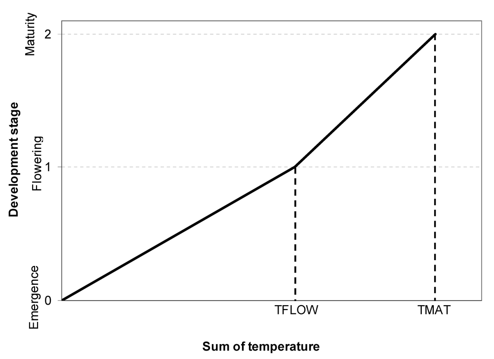
Figure 7.3. Schematic relationship between sum of temperature and development stage.
TFLOW: sum of temperature needed to reach the flowering development stage; TMAT: sum of temperature needed to reach the maturity development stage. The development stage scale is defined as 0 = emergence, 1 = flowering, and 2 = maturity
Photosynthesis
Photosynthesis allows the production of assimilates that are made available for plant growth, using radiation energy. The computation of the rate of growth (RG) according to photosynthesis can be done in a synthetic way (e.g., Van Keulen et al., 1982; Sinclair and Muchow, 1999) as:
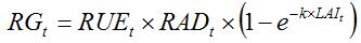 | (7.5) |
where
RAD is the daily global solar radiation;
RUE is the radiation use efficiency (Monteith, 1977; Sinclair and Muchow, 1999), that is, the amount of assimilates produced per quantity of radiation intercepted by the canopy. The term [1 - exp(-k × LAI)] is the proportion of light intercepted by the crop, following Beer’s law; and
k is the coefficient of light extinction. Note that equation (7.5) reflects the same processes embedded in the framework developed by Monteith (equation 7.2).
Crop growth models developed to address crop physiological processes at a finer level of detail have incorporated respiration and transpiration (to, e.g., analyze the effects of water stress or of pests affecting transpiration; e.g., Penning de Vries et al., 1989; Goudriaan and van Laar, 1994). Here, the approach using
RUE is used, because it allows capturing and analyzing in a synthetic way a number of physiological processes in crop growth.
LAI can be computed from the dry biomass of leaves (LEAFB):
|
LAIt =
SLAt x
LEAFBt | (7.6) |
where
SLA is the specific leaf area (i.e., the leaf area per unit of leaf dry biomass) and is a function of the crop development stage. Young leaves are in general thinner, and thus have a higher
SLA than older leaves. It is therefore expected that
SLA declines over time.
Radiation use efficiency, RUE, represents the overall efficiency of the crop to convert plant biomass from intercepted light.
RUE thus encapsulates the efficiency of several processes: gross photosynthesis, respiration, transportation of photosynthates before on-site biosynthesis, and synthesis of complex molecules from photosynthates (e.g., proteins, lipids, polysaccharides).
RUE varies depending on (1) the efficiency of photosynthesis, which depends on the concentration of leaf N and on water availability (Penning de Vries et al., 1989), and; (2) the respective proportion of the different types of organic components synthesized from photosynthates: the energy required for the biosynthesis of a given compound depends on the type of organic group it belongs to (Penning de Vries et al., 1989). For example, lipids require much more energy (that is, more glucose) to be synthesized than carbohydrates, the proteins being in an intermediate position (Penning de Vries et al., 1989). The proportion of compounds synthesized depends on the crop development stage.
Thus,
RUE varies depending on the crop species, on the crop development stage, and on nutrients and water supply of a crop (Sinclair and Muchow, 1999).
The amount of assimilates that are made available for plant growth (POOL) is accumulated daily at the rate of growth,
RG:
|
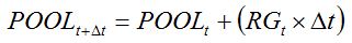 | (7.7) |
Partitioning of assimilates
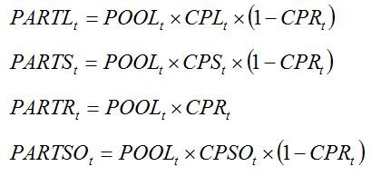
Assimilates that are accumulated daily are partitioned to the different plant organs. Most crop plants develop four broad types of organs: leaves, stems, roots, and storage organs (e.g., grains, tubers). The increase in dry biomass of the different crop organs can be computed as follows:
|
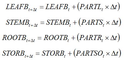 | (7.8)
(7.9)
(7.10)
(7.11) |
where
PARTL,
PARTS,
PARTR, and
PARTSO are the daily flows of assimilates towards leaves, stems, roots, and storage organs, respectively. These flows depend on coefficients of partitioning, which in turn depend on the development stage:
|
 | (7.12)
(7.13)
(7.14)
(7.15) |
where
CPL,
CPS,
CPR, and CPSO are the partitioning coefficients of assimilates to leaves, stems, roots, and storage organs, respectively, at the development stage at date
t. CPL,
CPST, and
CPSO represent partitioning coefficients relative to the biomass partitioned above ground. CPR represents the coefficient of partitioning towards roots, relative to the total plant biomass.
Assimilates produced by photosynthesis are therefore partitioned towards the plant organs, and equation (7.7) becomes:
|
 | (7.16) |
In general, partitioning towards roots, stems, and leaves occurs until flowering. From this stage onwards, most, if not all, assimilates are partitioned towards the storage organs (Fig. 7.4).
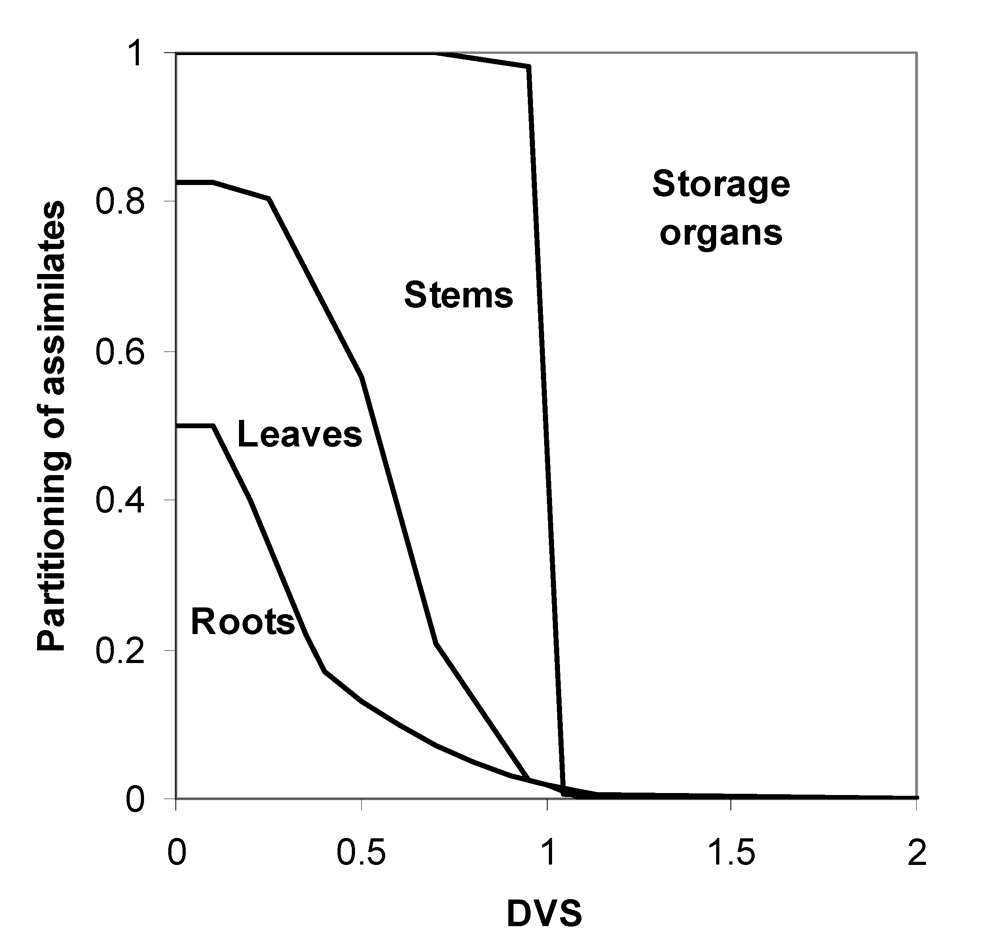
Figure 7.4. Typical dynamics of partitioning of assimilates towards the different organs in the case of a cereal.
Leaf senescence
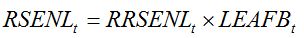
Leaf senescence refers to physiological ageing and occurs towards the end of the crop cycle. Leaf senescence can be represented by a loss of leaf dry biomass (RSENL), which can be made proportional to a relative rate of leaf senescence (RRSENL) and to the dry biomass of leaves (LEAFB), with
RRSENL depending on the development stage.
|
 | (7.17) |
Thus equation (7.8) becomes:
|
 | (7.18) |
Accumulation and redistribution of reserves
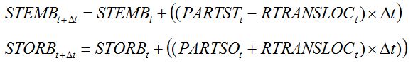
Carbohydrates can be stored in stems or roots before being translocated towards storage organs (Penning de Vries et al., 1989). In the case of cereals, this can be translated in a simple way by simulating a flow of biomass from the stems towards the storage organs after flowering. Equations (7.9) and (7.11) thus become:
|
 | (7.19)
(7.20) |
where
RTRANSLOCt is the daily rate of translocation of starch from stems to storage organs.
RTRANSLOCt varies with the development stage, and is proportional to the dry biomass of stem at flowering.
Dynamics of tillers (or shoots)
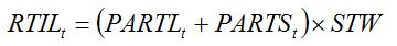
In the following, we shall refer to tillers or plant shoots in an equivalent manner, as GENECROP can be used equivalently for a cereal (where the aerial part of a plant ― the unit of a crop stand ― consists of tillers as sub-units) or a dicotyledon (where shoots could be considered instead as sub-units) crop. Crop growth simulation models do not usually consider the dynamics of plant sub-units, since consideration of the functioning of a system's unit is sufficient to understand the behavior of the system at the higher level of integration (Penning de Vries and Van Laar, 1982). When aiming at simulating the effects of pest injuries on crop growth, however, the simulation of tiller (or shoot) dynamics may allow direct and relevant simulation of the way injuries affect tiller (shoot) mortality. The tiller (shoot) dynamic can be modeled by considering first vegetative tillers (shoots), which multiply during the tillering (shoot emission) phase. The tillering rate is assumed to be proportional to the rates of leaf and stem growth:
|
 | (7.21) |
where
RTIL is the tillering rate;
PARTL is the rate of leaf growth;
PARTS is the rate of stem growth;
STW is the dry biomass of one new tiller.
During the tillering phase, leaf and stem growth contribute progressively less to generating new tillers, and more to leaf production, leaf expansion, and stem elongation. Tiller production is therefore seen in the model to compete with tiller growth, with respect to assimilate allocation to stems and leaves. This is reflected by introducing the factor (1-(VTIL/MAXTIL)) in equation (7.21), where
VTIL and
MAXTIL represent the number of vegetative tillers and the maximum number of tillers, respectively. Tillering is furthermore governed by crop development: when the crop reaches the maximum tillering stage, assimilates are not allocated for tillering any more. This is reflected by a multiplicative term,
DVE, which is made dependent on development stage. Equation (7.21) thus becomes:
|
 | (7.22) |
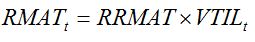
The shift from the vegetative phase to the reproductive phase corresponds to the maturation of vegetative tillers (shoots), which become reproductive. This is reflected by a rate of maturity (RMAT; which depends on development stage), which flows from the number of vegetative tillers (VTIL) to the number of reproductive tillers (REPTIL):
|
 | (7.23) |
where
RRMAT is the relative rate of tiller maturity.
A fraction of the vegetative tillers,
FST, may remain vegetative and not produce any storage organ. Furthermore, between maximum tillering and flowering stages, some of the younger tillers die, due to competition for light and nutrients with the other tillers. The dynamics of vegetative tillers and of reproductive tillers is described by equations (7.24) and (7.25), respectively:
|
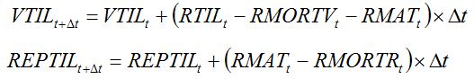 | (7.24) (7.25) |
with:
|
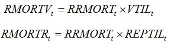 | (7.26) (7.27) |
where
RRMORTt is the relative rate of tiller mortality, and depends on development stage.
Model parameters
The simulation starts at 15 days after crop establishment (DACE), and ends when DVS reaches 2. Model inputs and parameters have been chosen to be within the range of values found for crops (or cereals) under favorable environments.
Weather variables used as inputs (driving functions) are daily minimum and maximum temperature (which drive the development stage) and daily radiation (which drives the rate of crop growth). Minimum and maximum temperature have been set to 24°C and 30°C, respectively, and are kept constant over the duration of the simulation for the sake of simplicity. Global radiation is also constant over time, and has been set to 17 mJ·m-2·day-1.
Parameters for crop development have been set to 1500°C·day and 2000°C·day for
TFLOW and
TMAT, respectively, and to 8°C for
TBASE (threshold temperature under which the crop does not develop). The main parameters for crop growth have been set to the following values:
RUE = 1.2 g·MJ-1 (value for a crop under favorable conditions; Monteith, 1977; Sinclair and Muchow, 1999)
k = 0.6 (value for a canopy with erect leaves; Goudriaan, 1977)
SLA decreases from 0.037 to 0.018 m2·g-1 from emergence (DVS=0) to flowering (DVS=1), and from 0.018 to 0.017 m2·g-1 from flowering to maturity (derived from Willocquet et al., 2004).
Coefficients of partitioning towards the different organs according to the development stage are derived from Willocquet et al. (2004). The maximum number of tillers has been set to 900 tillers·m-2.
Simulations
The STELLA model GENECROP.STMX will allow you to:
- explore the model structure and equations,
- explore the model inputs,
- explore the model outputs, and
- run the model with varying values of
RUE, so as to observe the effects these changes have on the dynamics of the crop growth and on final yield.
The simulated crop growth using GENECROP is displayed in Fig. 7.5.
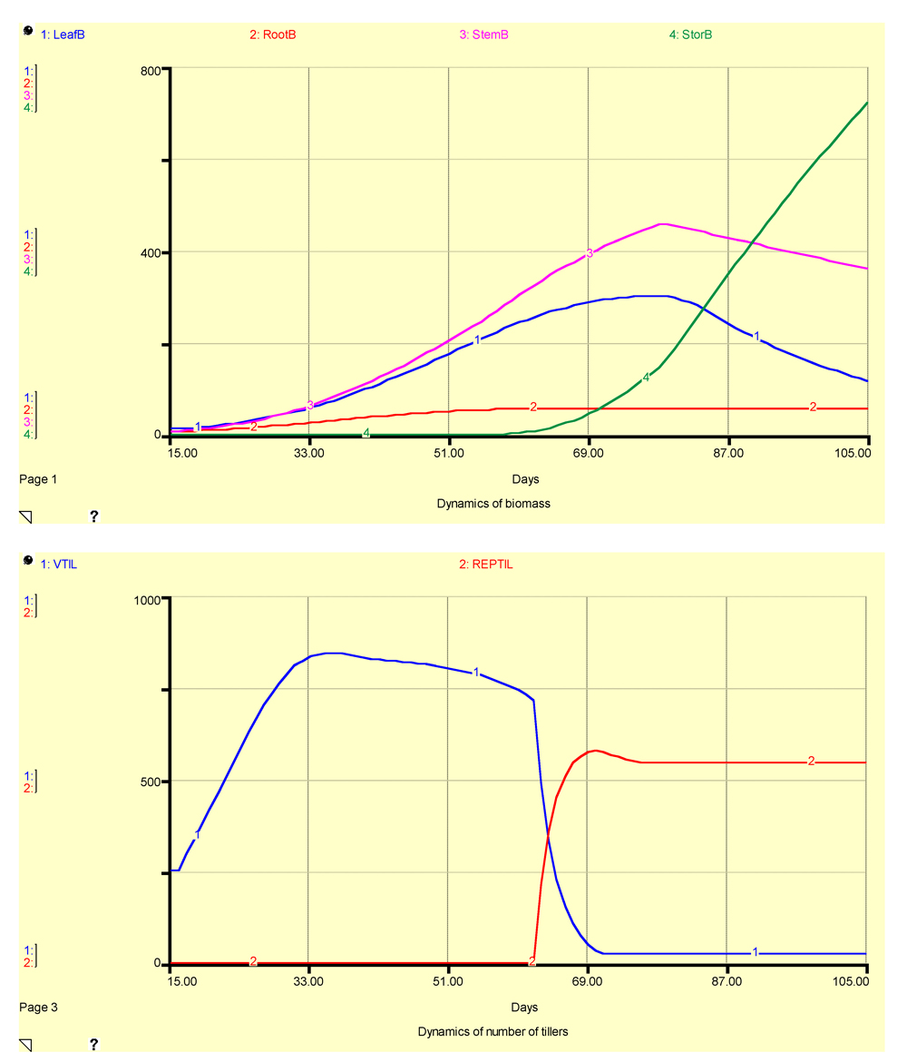
Figure 7.5. Simulated outputs of biomass (upper graph) and number of tillers (lower graph) using GENECROP
The model outputs reflect the hypotheses captured in the different equations of the model. Crop reaches maturity when DVS equals 2, that is, at 105 days after crop establishment (DACE). The biomass of roots increases regularly until 51 DACE, then tapers off at around 60 DACE. Leaf biomass increases according to a sigmoid-like shape until flowering (which occurs at 77 DACE), and then declines as leaf senescence takes place. Stem biomass increases regularly until flowering, and then declines nearly linearly as carbohydrates are translocated towards the storage organs. The dry biomass of storage organs increases exponentially, and then nearly linearly, when all assimilates are partitioned towards these organs towards the end of the crop cycle. The final yield is about 700 g·m-2, that is, 7 t·ha-1.
The number of vegetative tillers increases until maximum tillering, then decreases because of tiller mortality due to competition, and finally decreases because vegetative tillers become reproductive. The number of reproductive tillers increases when vegetative tillers reach the reproductive stage, and then remains at the same level until the end of the crop cycle, about 500 tillers·m-2.
Concluding remarks
The reader will have noticed that this chapter deals with annual crops, with a definite tinge towards cereals. This is a reflection of the authors' main interest, but mainly because such systems are comparatively simple. Complication (but not necessarily complexity) may emerge when:
- one considers crops whose lifespan is long and/or covers several seasons, such as cassava, sugarcane, alfalfa, pyrethrum, or banana;
- the focus of research concerns perennials, e.g., fruit trees, grapevine, or blueberries;
- crop species or genotypes with indeterminate growth are considered, such as tomatoes or beans.
Many of the ideas that have been forwarded in this chapter are relevant to such crops, however. One, in particular, is the remobilization of carbohydrates from one season to the other, which, for example, explains the yearly oscillations of coffee yield in a plantation, the associated variation of coffee susceptibility to rust, and so, the yearly oscillations of coffee rust epidemics (Avelino et al., 2004).
Summary
This chapter describes:
- The RI-RUE concept.
- The main processes involved in crop growth.
- How they are captured in a quantitative and dynamic way into a generic simulation model, GENECROP.
- The equations, parameters, and flowchart of GENECROP.
- Includes the STELLA file, which can be used to explore the model structure and the effect of some parameters on the simulated dynamics of the model variables.
References
Avelino, J., Willocquet, L., and Savary, S. 2004. Effects of crop management patterns on coffee rust epidemics. Plant pathology 53: 541-547.
Goudriaan, J. 1977. Crop Micrometeorology: a Simulation study. Simulation Monographs. Pudoc, Wageningen.
Goudriaan, J., and van Laar, H. H. 1994. Modelling Potential Crop Growth Processes. Kluwer Academic Publishers, Dordrecht.
Johnson K. B., Johnson S. B., and Teng, P. S. 1986. Development of a simple potato growth model for use in crop-pest management. Agric. Sys. 19:189-209.
Kiniry, J. R., Bean, B., Xie, Y., and Chen, P. 2004. Maize yield potential: critical processes and simulation modeling in a high-yielding environment. Agric. Sys. 82:45-56.
Monsi, M., and Saeki, T. 1953. Uber den Lichtfaktor in den Pflanzengesellschaften und sein Bedeutung für die Stoffproduktion. Jpn. J. Bot. 14:22-52.
Monteith, J. L. 1977. Climate and the efficiency of crop production in Britain. Phil. Trans. Roy. Soc. Lond. 281:277-294.
Penning de Vries, F. W. T., Jansen, D. M., ten Berge, H. F. M., and Bakema, A., eds. 1989. Simulation of Ecophysiological Processes of Growth in Several Annual Crops. IRRI, Los Baños, and Pudoc, Wageningen.
Penning de Vries, F. W. T., and Van Laar, H. H. 1982. Simulation of Plant Growth and Crop Production. Pudoc, Wageningen.
Richter, G. M., Haggard, K. W., and Mitchell, R. A. C. 2001. Modelling radiation interception and radiation use efficiency for sugar beet under variable climatic stress. Agric. Forest Meteorol. 109:13-25.
Sinclair, T. R. 1986. Water and nitrogen limitations in soybean grain production. I. Model development. Field Crops Res. 15:125-141.
Sinclair, T. R., and Muchow, R. C. 1999. Radiation-use efficiency. Adv. Agron. 65:215-265.
Steer, B. T., Milroy, S. P., and Kamona R. M. 1993. A model to simulate the development, growth and yield of irrigated sunflower. Field Crops Res. 32:83-99.
Thornley, J. H. M., and France, J. 2007. Mathematical Models in Agriculture. Quantitative Methods for the Plant, Animal and Ecological Sciences, 2nd ed. CABI, Wallingford.
Van Keulen, H., Penning de Vries, F. W. T., and Drees, E. M. 1982. A summary model for crop growth. Pages 87-97 in: Simulation of Plant Growth and Crop Production. F. W. T. Penning de Vries and H. H. van Laar, eds. Pudoc, Wageningen.
Whisler, F. D., Acock, B., Baker, D. N., Fye, R. E., Hodges, H. F., Lambert, J. R., Lemmon, H. E., McKinion, J. M., and Reddy, V. R. 1986. Crop simulation models in agronomic systems. Adv. Agron. 40:141-208.
Willocquet, L., Elazegui, F. A., Castilla, N., Fernandez, L., Fischer, K. S., Peng, S., Teng, P. S., Srivastava, R. K., Singh, H. M., Zhu, D., and Savary, S. 2004. Research priorities for rice pest management in tropical Asia: a simulation analysis of yield losses and management efficiencies. Phytopathology 94:672-682.
Yin, X., Struik, P. C., and Kropff, M. J. 2004. Role of crop physiology in predicting gene-to-phenotype relationships. Tr. Plant Sci. 9:427-432.
Suggested reading
Charles-Edwards, D. A., Doley, D., and Rimmington, G. M. 1986. Modelling Plant Growth and Development. Academic Press, Sydney.
Sinclair, T. R., and Seligman, N. G. 1996. Crop modeling: from infancy to maturity. Agron. J. 88: 698-704.
van Ittersum, M. K., Leffelaar, P. A., van Keulen, H., Kropff, M. J. Bastiaans, L., and Goudriaan, J. 2003. On approaches and applications of the Wageningen crop models. Eur. J. Agron. 18:201-234.
Exercises and questions
1. What is the difference between (crop) growth and development?
2. What is the dimension of a rate of crop growth? What is the dimension of a rate of crop development?
3. The increase in crop biomass directly depends on several factors, including
- leaf biomass
- radiation
- LAI
- temperature
4. Radiation Use Efficiency, RUE can be expressed with the unit(s)
- [g.MJ-1.m-2]
- [g.MJ-1 ]
- [MJ.g-1.m-2]
- [g.MJ-1.m-2.day-1]
5. Crop development
- represents changes in crop biomass
- mainly depends on temperature
- mainly depends on radiation
- determines the partitioning of assimilates towards plant organs
Answers to exercises and questions
1. Crop growth is the accumulation (and possibly decrease) of biomass over time; whereas crop development represents the passing of a crop (seen as a cohort, i.e., a population of plants which have a similar development stage at a given point of time) through the successive development stages of its life cycle. For instance, in cereals, development spans from seeds and their germination, to ripening of ears.
2. The rate of crop growth is measured as a quantity of biomass [M] per unit time [T], so a rate of crop growth is measured as: [M.T-1]. Development is, by essence, a qualitative attribute, and so does not have dimension [ - ], so a rate of development is [T-1].
3. b: radiation, and c: LAI.
4. b: [g.MJ-1 ].
5. b: mainly depends on temperature, and d: determines the partitioning of assimilates towards plant organs.
Appendix 7.1. Program listing of GENECROP
LeafB(t) = LeafB(t - dt) + (PartL - RSenL) * dt
INIT LeafB = 10
INFLOWS:
PartL = CPL*Pool
OUTFLOWS:
RSenL = rrsen*LeafB
MaxStemb(t) = MaxStemb(t - dt) + (rmaxstemb) * dt
INIT MaxStemb = 6
INFLOWS:
rmaxstemb = PartLS
Pool(t) = Pool(t - dt) + (RGrowth - PartS - PartL - PartSO - PartR) * dt
INIT Pool = 0
INFLOWS:
RGrowth = RAD*RUE*(1-EXP(-k*LAI))
OUTFLOWS:
PartS = CPS*Pool
PartL = CPL*Pool
PartSO = CPP*Pool
PartR = CPR*Pool
REPTIL(t) = REPTIL(t - dt) + (Rmat - Rmortr) * dt
INIT REPTIL = 0
INFLOWS:
Rmat = if DVS<0.8 or DVS>1 then 0 else if VTIL
OUTFLOWS:
Rmortr = rrmort*REPTIL
RootB(t) = RootB(t - dt) + (PartR) * dt
INIT RootB = 5
INFLOWS:
PartR = CPR*Pool
StemB(t) = StemB(t - dt) + (PartS - RTransloc) * dt
INIT StemB = 6
INFLOWS:
PartS = CPS*Pool
OUTFLOWS:
RTransloc = IF(DVS>1) then ddist else 0
STEMP(t) = STEMP(t - dt) + (Dtemp) * dt
INIT STEMP = 320
INFLOWS:
Dtemp = ((TMAX+TMIN)/2)-TBASE
StorB(t) = StorB(t - dt) + (PartSO + RTransloc) * dt
INIT StorB = 0
INFLOWS:
PartSO = CPP*Pool
RTransloc = IF(DVS>1) then ddist else 0
VTIL(t) = VTIL(t - dt) + (Rtil - Rmat - Rmrtv) * dt
INIT VTIL = 250
INFLOWS:
Rtil = PartLS*STW*(1-(VTIL/Maxtil))*DVE
OUTFLOWS:
Rmat = if DVS<0.8 or DVS>1 then 0 else if VTIL
Rmrtv = (rrmort*VTIL)
CPL = CPPL*(1-CPR)
CPP = CPPP*(1-CPR)
CPS = (1-CPL-CPP)*(1-CPR)
ddist = 0.005*MaxStemb
DVS = if stemp
FST = 0.05
k = 0.6
LAI = LeafB*SLA
Maxtil = 900
PartLS = PartL+PartS
RAD = 17
RRMAT = 0.3
RUE = 1.2
STW = 20
TBASE = 8
TFLOW = 1500
TMAT = 2000
TMAX = 30
TMIN = 24
Totil = VTIL+REPTIL
CPPL = GRAPH(DVS)
(0.00, 0.55), (0.1, 0.536), (0.2, 0.521), (0.3, 0.507), (0.4, 0.493), (0.5, 0.479), (0.6, 0.464), (0.7, 0.45), (0.8, 0.3), (0.9, 0.15), (1, 0.00), (1.10, 0.00), (1.20, 0.00), (1.30, 0.00), (1.40, 0.00), (1.50, 0.00), (1.60, 0.00), (1.70, 0.00), (1.80, 0.00), (1.90, 0.00), (2.00, 0.00)
CPPP = GRAPH(DVS)
(0.00, 0.00), (0.05, 0.00), (0.1, 0.00), (0.15, 0.00), (0.2, 0.00), (0.25, 0.00), (0.3, 0.00), (0.35, 0.00), (0.4, 0.00), (0.45, 0.00), (0.5, 0.00), (0.55, 0.00), (0.6, 0.00), (0.65, 0.00), (0.7, 0.00), (0.75, 0.00), (0.8, 0.143), (0.85, 0.286), (0.9, 0.429), (0.95, 0.571), (1.00, 0.714), (1.05, 0.857), (1.10, 1.00), (1.15, 1.00), (1.20, 1.00), (1.25, 1.00), (1.30, 1.00), (1.35, 1.00), (1.40, 1.00), (1.45, 1.00), (1.50, 1.00), (1.55, 1.00), (1.60, 1.00), (1.65, 1.00), (1.70, 1.00), (1.75, 1.00), (1.80, 1.00), (1.85, 1.00), (1.90, 1.00), (1.95, 1.00), (2.00, 1.00)
CPR = GRAPH(DVS)
(0.00, 0.3), (0.1, 0.263), (0.2, 0.225), (0.3, 0.188), (0.4, 0.15), (0.5, 0.112), (0.6, 0.075), (0.7, 0.038), (0.8, 0.00), (0.9, 0.00), (1, 0.00), (1.10, 0.00), (1.20, 0.00), (1.30, 0.00), (1.40, 0.00), (1.50, 0.00), (1.60, 0.00), (1.70, 0.00), (1.80, 0.00), (1.90, 0.00), (2.00, 0.00)
DVE = GRAPH(DVS)
(0.00, 1.00), (0.4, 1.00), (0.8, 0.00), (1.20, 0.00), (1.60, 0.00), (2.00, 0.00)
rrmort = GRAPH(DVS)
(0.00, 0.00), (0.1, 0.00), (0.2, 0.00), (0.3, 0.00), (0.4, 0.00), (0.5, 0.02), (0.6, 0.02), (0.7, 0.02), (0.8, 0.02), (0.9, 0.02), (1, 0.00), (1.10, 0.00), (1.20, 0.00), (1.30, 0.00), (1.40, 0.00), (1.50, 0.00), (1.60, 0.00), (1.70, 0.00), (1.80, 0.00), (1.90, 0.00), (2.00, 0.00)
rrsen = GRAPH(DVS)
(0.00, 0.00), (0.1, 0.00), (0.2, 0.00), (0.3, 0.00), (0.4, 0.00), (0.5, 0.00), (0.6, 0.00), (0.7, 0.00), (0.8, 0.00), (0.9, 0.00), (1, 0.00), (1.10, 0.013), (1.20, 0.026), (1.30, 0.04), (1.40, 0.04), (1.50, 0.04), (1.60, 0.04), (1.70, 0.04), (1.80, 0.04), (1.90, 0.04), (2.00, 0.04)
SLA = GRAPH(DVS)
(0.00, 0.037), (1.00, 0.018), (2.00, 0.017)

