Reproductive systems can be asexual (by mitosis), sexual (by meiosis) or a mixture of sexual and asexual reproduction (Figure 14). All bacteria and viruses exhibit asexual reproduction. Fungi and Oomycetes can be asexual, sexual, or exhibit a mixture of both types of reproduction.
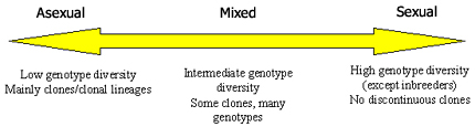 |
| Figure 14. The range of possible pathogen reproductive systems and expected effects on degree of clonality with pathogen populations. |
Mating systems are relevant only for organisms that undergo sexual reproduction. The possible mating systems span a continuum that ranges from 100% inbreeding to 100% outcrossing.
Mating and reproductive systems affect the way that alleles are combined in individuals in a population. Outcrossing organisms put together new combinations of genes rapidly, leading to many different genotypes within populations (and creating high genotype diversity) and the potential for rapid adaptation in a changing environment. If an organism is an obligate outcrosser, then frequent recombination will break up coadapted combinations of alleles each generation, which may be disadvantageous for a pathogen if the environment is constant and stable.
Pathogens that are inbreeding or that undergo asexual reproduction tend to keep together old combinations of genes, leading to lower genotypic diversity in populations. If a well-adapted genotype (containing a coadapted combination of alleles) exists and the organism is an inbreeder or asexual, it has the potential to keep together the coadapted combination of alleles for a long time. But if the environment changes quickly, these organisms take longer to put together new combinations of alleles that allow them to optimize their adaptation to a new environment.
Pathogens that have "mixed" reproductive/mating systems, including both sexual and asexual reproduction, potentially benefit from the advantages inherent in both types of reproduction. Recombination that occurs during sexual reproduction puts together new combinations of alleles that can be tested in the local environment, and asexual reproduction combined with selection can maintain the allele combinations that are best adapted to the local environment.
Fungi are especially flexible with regard to the possible ways they can mate and reproduce. Bacteria and viruses can recombine without meiosis, but their reproductive system is obligately asexual.
Mating systems are often considered in terms of the amount of inbreeding that occurs in populations of sexual organisms. The inbreeding coefficient (often abbreviated as F) is also called the fixation index. F is the probability that the two alleles of a gene pair in a diploid individual are identical by descent, meaning that they were derived from a common ancestor in past generations.
 |
|
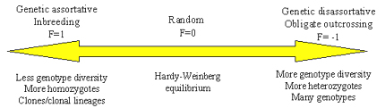
Figure 15. The range of possible pathogen mating systems and expected effects on degree of homozygosity, heterozygosity and genotype diversity within pathogen populations.
|
At one end of the mating system scale (F=1), we have genetic assortative mating (Figure 15). Organisms with assortative mating systems tend to mate with individuals that share alleles, like close relatives. An extreme example of genetic assortative mating is inbreeding, which occurs for many plants that self-fertilize. For strictly inbreeding plants, F=1. It is likely that some pathogens also experience inbreeding. For example, many smut fungi may be forced to undergo brother-sister mating because a dikaryon must form for successful infection, and the most likely encounter between strains of opposite mating type in the soil will be basidiospores that emerge from the same probasidium. Another example is homothallic fungi that can self-fertilize. The result of genetic assortative mating is a population structure characterized by an excess of homozygotes (compared to the predictions of Hardy-Weinberg equilibrium) and a relatively low level of genotypic diversity. Many cycles of inbreeding will establish clonal lineages in these populations.
At the other end of the scale, we have genetic disassortative mating. Organisms with disassortative mating systems tend to mate with individuals that do not share alleles, meaning that they have no common ancestors. An extreme example of genetic disassortative mating is shown by plants and fungi that are obligate outcrossers as a result of a mating incompatibility system. For example, some plant pathogens that are basidiomycete fungi, such as Armillaria spp. have tetrapolar mating systems that prevent them from self-fertilizing. The result of genetic disassortative mating is a population structure characterized by an excess of heterozygotes and a high degree of genotypic diversity.
In the middle of the mating scale, we have random mating. Organisms with random mating tend to mate at random with other individuals in the population. Human populations exhibit random mating. The result of random mating is Hardy-Weinberg equilibrium. The observed frequencies of homozygotes and heterozygotes for any locus matches the predicted frequencies under the assumption that gametes unite randomly to form zygotes. Another result of random mating is random association among alleles at different loci in haploid organisms, a state called gametic equilibrium.
Mating systems have been studied for several fungal plant pathogens. For diploid oomycetes such as Phytophthora spp., mating systems range from inbreeding to outcrossing as indicated by fixation indices ranging from 1.0 to -0.82 (Table 3). Departures from Hardy-Weinberg equilibrium cannot be measured for haploid pathogens. In these cases departures from gametic equilibrium are used to indicate mating systems. Examples of plant pathogens that appear to mate at random according to measures of gametic equilibrium are the wheat pathogens Phaeosphaeria nodorum and Mycosphaerella graminicola (Chen and McDonald 1996; Keller et al. 1997). Randomly mating populations often have a high degree of genotypic diversity. But if the level of gene diversity in the population is low, e.g. because the population originated from a small number of individuals (founder effect), genotypic diversity may be low even if the population is randomly mating.
|
Species |
Sample
Size |
No. of
Loci |
Heterozygosity |
Fixation
Index |
| Actual |
Expected |
|
Homothallic species |
|
P. boehmeriae |
11 |
12 |
0.015 |
0.32 |
0.95 |
|
P. cactorum |
47 |
18 |
0.056 |
0.037 |
-0.51 |
|
P. citricola |
125 |
14 |
0.007 |
0.279 |
0.97 |
|
P. heveae |
14 |
17 |
0.05 |
0.16 |
0.69 |
|
P. katsurae |
16 |
17 |
0.00 |
0.11 |
1.0 |
|
P. sojae |
48 |
15 |
0.00 |
— |
1.0 |
|
|
|
|
|
|
|
|
Heterothallic species |
|
|
|
|
|
|
P. botryosa |
10 |
18 |
0.006 |
0.08 |
0.93 |
|
P. cambivora |
25 |
18 |
0.060 |
0.071 |
0.15 |
|
P. capsici |
84 |
18 |
0.019 |
0.20 |
0.91 |
|
P. cinnamomi |
|
|
|
|
|
|
Worldwide |
81 |
18 |
0.098 |
0.134 |
0.27 |
|
Australia |
165 |
20 |
0.010 |
0.049 |
0.80 |
|
Australia |
280 |
19 |
0.051 |
0.115 |
0.56 |
|
PNG |
18 |
20 |
0.058 |
0.088 |
0.34 |
|
P. citrophthora |
43 |
18 |
0.107 |
0.20 |
0.47 |
|
P. infestans |
|
|
|
|
|
|
Mexico |
50 |
15 |
0.037 |
0.046 |
0.20 |
|
non-Mexican |
46 |
15 |
0.120 |
0.066 |
-0.82 |
|
P. meadii |
33 |
18 |
0.066 |
0.12 |
0.45 |
|
P. megakarya |
15 |
17 |
0.078 |
0.19 |
0.59 |
|
P. palmivora |
|
|
|
|
|
|
Worldwide |
106 |
17 |
0.111 |
0.08 |
-0.39 |
|
East Asia |
62 |
17 |
0.135 |
0.122 |
-0.11 |
|
P. parasitica |
60 |
19 |
0.079 |
0.11 |
0.28 |
Table 3. Fixation indices for 15 species of Phytophthora (Goodwin 1997).
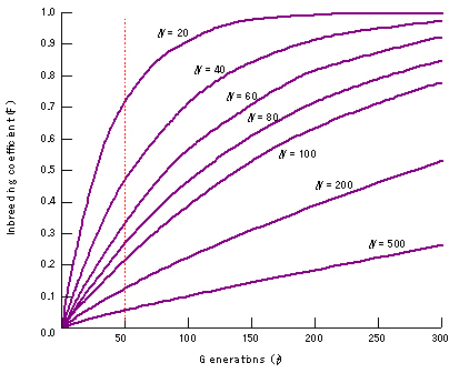
As the effective population size (Ne) of a population becomes smaller (for example as a result of a bottleneck or a founder event), it becomes more likely that individuals in a population will mate with relatives. As a result, small populations experience an increased degree of inbreeding (F increases) with subsequent higher levels of homozygosity, and lower levels of genotypic diversity. Plant and animal breeders use this principle to fix desirable alleles in populations of domesticated animals and plants. The expected increase of the inbreeding coefficient F in populations with different effective size over time is shown in Figure 16. Populations may exhibit inbreeding depression if Ne becomes too small. Inbreeding depression results from having deleterious recessive alleles that become homozygous (hence are expressed) in inbreeding populations. Inbreeding depression is of great concern for wild animals on the brink of extinction. Inbreeding depression has been hinted at in Phytophthora infestans (Shattock et al. 1986), but has not been conclusively demonstrated for plant pathogens, perhaps because nobody has studied it thus far.
 |
|
Figure 16. The relationship between effective population size and fixation index. Small populations become inbred more rapidly than large populations, often leading to inbreeding depression. After 50 generations, F=0.70 for an effective population size of 20 individuals, while F=0.05 for a population of 500 individuals. |
Because organisms with a sexual cycle undergo meiosis, recombination takes place that shuffles together new combinations of alleles with each sexual cycle. This leads to high levels of genotypic diversity in sexual populations compared to asexual populations. It is thought that sexual reproduction and the consequent independent assortment of genes produces a population that is able to adapt more quickly to a changing environment than an equivalent asexual or inbreeding population. But organisms with regular sexual reproduction are less likely to form coadapted gene complexes that can optimize fitness in a stable environment.
The discussion on mating systems is relevant only for organisms that have a component of sexual reproduction in their life cycles. Many pathogens utilize asexual reproduction (through mitosis), giving rise to a number of clones. Clonal reproduction is extremely important for many plant pathogens. For most pathogens, it is the propagules produced by asexual reproduction that cause epidemics that do the most damage. Pathogens that reproduce exclusively asexually tend to have a population structure in which genetic diversity is arrayed in a limited series of clones, or clonal lineages. These clones may become widely disseminated as a result of human activities. In theory, we expect that strictly asexual organisms will have a limited potential to adapt to a changing environment, and their evolutionary potential is limited to the random mutations that occur within a clonal lineage. But in a stable and homogeneous environment, like a farmer's field planted to a genetically uniform monoculture, any genotype that possesses a coadapted combination of genes that is very fit in the agroecosystem (able to infect and reproduce on the planted cultivar) will have an advantage over equivalent pathogens that undergo sexual reproduction (which will break up the coadapted complex of alleles).
Many pathogenic fungi can undergo a combination of sexual and asexual reproduction. We can refer to this as a mixed reproduction system. Pathogens with mixed reproduction systems have the best of both worlds. Sexual reproduction can create new combinations of alleles that allow the pathogen to track changes in the environment. And asexual reproduction can operate to keep together a good combination of alleles after it arises. These are probably the most dangerous pathogens in agroecosystems because they have the greatest potential for rapid evolution.
Genetic diversity has two components, namely gene diversity and genotypic diversity. Gene diversity refers to the diversity for alleles (ultimately due to differences in DNA sequence) for a specific gene, or locus, on a chromosome. Gene diversity is best measured using multiallelic neutral genetic markers such as isozymes, RFLPs, microsatellites, or single nucleotide polymorphisms (SNPs). But it also can be measured using dominant genetic markers such as Amplified Fragment Length Polymorphism (AFLP).
Genotypic diversity refers to the diversity in the combinations of alleles that occurs across all loci that are assayed. In other words, genotypic diversity is based on the number of genetically distinct individuals in a population and their frequencies. Measures of genotypic diversity are meaningless for organisms like humans that exhibit only random mating, because each human (with the exception of identical twins) is genetically different, hence genotypic diversity is always at its maximum value. But genotypic diversity is very important for asexual pathogens or pathogens with mixed reproduction systems. Genotypic diversity is often measured using DNA fingerprinting methods or by constructing multilocus genotypes for each individual in a population.
A comparison of gene and genotype diversity:
Quantitative measures of gene diversity are based on the number of alleles per locus and the frequencies of alleles at each locus. Diversity increases as the number of alleles increases, and as the frequency of alleles becomes more evenly distributed. Gene diversity is affected by the type of genetic marker assayed (neutral markers are expected to show higher diversity than selected markers), the size of the population (larger populations experience less genetic drift and have more alleles), and the age of the population (older populations have had a longer time for mutation to occur and for genetic drift to increase the frequency of neutral mutations).
The most commonly used measure of gene diversity was proposed by Nei (1973). Nei's measure of gene diversity is calculated for each locus as h = 1-  xj2, where xj is the frequency of the jth allele at the locus. For a diploid population at Hardy-Weinberg equilibrium, this measure of gene diversity is the same as the expected frequency of heterozygotes at a locus, hence the measure is often called heterozygosity. But Nei showed that this measure could also be applied to haploid organisms and for non-random mating populations, and coined the term gene diversity for this measure. Nei's gene diversity is a measure of the probability that two copies of the same gene chosen at random in a population will have different alleles. These two genes could be chosen from the same, diploid individual (in this case a measure of heterozygosity) or from two haploid individuals in the same population (in this case a measure of gene diversity).
Quantitative measures of genotypic diversity are based on the number of genotypes and the frequencies of genotypes found in a population. Diversity increases as the number of genotypes increases and as the frequencies of genotypes become more evenly distributed. Genotype diversity is affected by the mating system (inbreeding organisms have lower genotype diversity than outcrossing), reproduction system (sexual organisms have higher diversity than asexual organisms), and selection. If one or two clones increase in frequency compared to other clones in a field population as a result of selection, the overall genotypic diversity of the selected population will decrease.
Thus, the reproductive/mating system will likely have a significant impact on genotypic diversity, but it does not necessarily have an impact on gene diversity. This can best be illustrated with an example as follows.
Measures of gene and genotype diversity should be based on sample sizes of at least 30 individuals per population. The following example includes only 8 individuals for the sake of brevity and clarity.
Consider two populations and three loci as follows:
Locus A has two alleles, A1 and A2. Locus B has two alleles B1 and B2. Locus C has two alleles C1 and C2. Consider the following two populations, which could represent two isolated populations of a haploid pathogen.
| Pop. 1 |
Pop. 2 |
A1 B1 C1
A1 B1 C2
A1 B2 C1
A1 B2 C2
A2 B1 C1
A2 B1 C2
A2 B2 C1
A2 B2 C2 |
A2 B1 C2
A2 B1 C2
A2 B1 C2
A2 B1 C2
A1 B2 C1
A1 B2 C1
A1 B2 C1
A1 B2 C1 |
| 8 genotypes |
2 genotypes |
|
|
f(A1) = f(A2) = 0.5
f(B1) = f(B2) = 0.5
f(C1) = f(C2) = 0.5 |
f(A1) = f(A2) = 0.5
f(B1) = f(B2) = 0.5
f(C1) = f(C2) = 0.5 |
In this case, the gene diversity is identical for the two populations because each has the same number of alleles at the same frequencies. Using Nei's measure, gene diversity is 0.50 for all three loci in both populations. But the genotypic diversities differ significantly, with Population 1 having all possible combinations of alleles at the two loci (8 genotypes total) and Population 2 having only two multilocus genotype combinations.
Sexual pathogen populations can reshuffle genetic variation very often, so new combinations of virulence alleles and fungicide resistance alleles can be generated quickly in sexual populations (as in Population 1). Asexual populations may have just as much gene diversity as sexual populations, but the diversity of alleles is distributed among clones or clonal lineages instead of among individuals (as in Population 2).
Dominant Polymerase Chain Reaction (PCR) -based genetic marker systems such as AFLP and RAPD that have only two alleles per locus have a maximum possible value for gene diversity of 0.50, which occurs when both alleles are present at equal frequency (Table 4). Thus it is not appropriate to compare genetic diversity in different pathogens if different marker systems (e.g. RFLPs and AFLPs) were used to collect data. The advantage of multiallelic systems such as RFLPs, microsatellites, or SNPs is that they can approach the theoretical maximum of 1.0 and they can provide additional information on gene diversity because of the presence of rare alleles or private alleles. Rare and private alleles can be used to identify centers of pathogen diversity and to monitor the movement of pathogen populations through time and space. But rare alleles may contribute only slightly to the overall measure of gene diversity (Table 5).
Number
of alleles |
Maximum
possible h |
| 2 |
0.50 |
| 3 |
0.67 |
| 4 |
0.75 |
| 5 |
0.80 |
| 6 |
0.83 |
| 7 |
0.86 |
Table 4. The number of alleles detected by a genetic marker system will affect Nei's measure of gene diversity (h). If only two alleles are detected, the maximum value for Nei's measure is 0.50. The maximum possible value for Nei's gene diversity is 1.0.
| Population |
Freq
allele 1 |
Freq
allele 2 |
Freq
allele 3 |
Nei's h |
| 1 |
0.50 |
0.50 |
0.00 |
0.50 |
| 2 |
0.40 |
0.60 |
0.00 |
0.48 |
| 3 |
0.30 |
0.70 |
0.00 |
0.42 |
| 4 |
0.20 |
0.80 |
0.00 |
0.32 |
| 5 |
0.10 |
0.90 |
0.00 |
0.18 |
| 6 |
0.01 |
0.99 |
0.00 |
0.02 |
| 7 |
0.02 |
0.96 |
0.02 |
0.08 |
| 8 |
0.05 |
0.90 |
0.05 |
0.19 |
| 9 |
0.33 |
0.34 |
0.33 |
0.67 |
Table 5. Nei's measure of gene diversity (h) according to the frequencies of two or three alleles. The maximum diversity possible in the three allele case is 0.67. Notice that the measure of diversity falls sharply once the frequency of the most common allele (allele 2 in this example) reaches 90%.
The previous discussion of mutation considered the effect of population size on the probability of simultaneous mutations from avirulence to virulence. The probability that two mutations would occur in the same individual (clone or clonal lineage) was extremely small. But what would occur if the pathogen also had a sexual cycle and could undergo recombination?
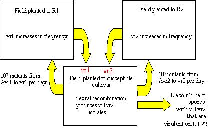
Returning to the previous example of Blumeria graminis f. sp. hordei, 1013 asexual spores can be produced per hectare per day. With a mutation rate of 10-6, there would be approximately 107 mutant spores produced in each hectare each day. The probability that a double mutant will occur is 10-12. But what is the chance that a recombinant will occur? This can best be illustrated with an example illustrated in Figure 17.
 |
|
Figure 17. Virulence alleles can recombine efficiently in agroecosystems where fields are arranged as a mosaic of susceptible cultivars and resistant cultivar with different resistance genes. This can lead to the breakdown of resistance gene pyramids.
|
Assume that two barley fields are planted to two cultivars that have different resistance genes, R1 and R2. A third nearby field is planted to a barley cultivar with no resistance genes (or a previously defeated resistance gene). The third field (susceptible) is the source of spores that initiate the infections.
From the susceptible field, we expect to find 107 mutants from avirulence to virulence for vr1 each day that can infect the field planted to R1. Only the vr1 mutants can survive on R1, so they increase in frequency quickly by asexual reproduction. Similarly, we expect that 107 mutants from avirulence to virulence for vr2 each day can infect the field planted to R2. Only the vr2 mutants survive, and these increase in frequency on R2. After the vr1 and vr2 types cause epidemics on R1 and R2, their spores can move back into the field of susceptible barley, possibly at quite high numbers. If the vr1 and vr2 mutants are in compatible mating types, they will have a chance to cross and recombine the vr1 and vr2 alleles during meiosis. While the number of successful matings between vr1 and vr2 mutants may represent only a small proportion of the matings in the population, if these genes are unlinked, then 25% of their progeny will contain both virulence alleles. These recombinants would be able to defeat a host genotype with both the R1 and R2 resistance genes.
A real-world experiment that illustrates the impact of sexual reproduction on the evolution of pathogen virulence is now underway. Phytophthora infestans, which was restricted to asexual reproduction as a single global lineage for more than 150 years, has recently become sexual (For more information search APSnet for P. infestans articles). Will it become more difficult to control now that new combinations of genes can come together in agricultural ecosystems? Keep in touch with the plant pathology literature!
Go to Knowledge Test for Interactions/Genetic Structure
Go to References
Next Section

