While measurements of the quantity of inoculum provide a good assessment of the progress of the epidemic, direct observation of inoculum is not always feasible or even possible. With most plant diseases, however, we can see some kind of symptoms that allow us to count the numbers of plants infected or estimate the amount of tissue infected. To be sure, there is a time lag between infection and the appearance of visible symptoms, and the manifestation of symptoms can be affected by the environmental conditions, but in general the progress of symptoms parallels the progress of inoculum production. Therefore, the same models that we have used to describe the buildup of inoculum also can be used to describe disease progress. We will follow the notation convention of Vanderplank (1963) and use x to represent the proportion of infected plants or the proportion of infected plant tissue. Using a dimensionless proportion between zero and one to represent disease makes the mathematics far simpler than using specific units, such as the total population of infected plants or the total area of infected tissue, for example.
Monocyclic Disease Progress
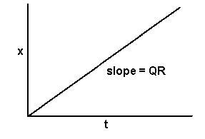
If disease progress in monocyclic epidemics is linear, the slope of the disease progress curve is constant. Furthermore, if disease progress in a monocyclic epidemic is proportional to the amount of initial inoculum (which is itself constant during the epidemic), we can make the slope of the disease progress curve the product of initial inoculum and a proportionality constant. Therefore, we can describe a monocyclic epidemic with linear disease progress using the differential equation:
dx/dt = QR
where dx is an infinitesimally small increment in the proportion of disease, dt is an infinitesimally small time step, Q is the amount of initial inoculum, and R is a proportionality constant that represents the rate of disease progress per unit of inoculum. Since Q and R are both constant during the course of an epidemic, the slope, dx/dt, is constant, and disease progress is linear. Just as with the K constant in the model of monocyclic inoculum production, R has a value that represents the "average" for the whole epidemic, a value that depends upon many factors, such as aggressiveness of pathogen, susceptibility of the host, the environmental conditions, etc. The units of Rare proportion per unit initial inoculum per unit time.
If we integrate the above differential equation, we get:
x = QRt
Graphically we see a straight line with an intercept of zero and a slope of QR
Polycyclic Disease Progress
In a model analogous to that of polycyclic inoculum production, the rate of change in disease is proportional to amount of disease at any point in time. Therefore, in differential form, the equation to describe polycyclic epidemics is:
dx/dt = xr
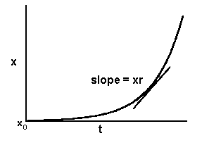
As with the monocyclic model, x is a dimensionless proportion between zero and one, and r is a constant that depends on the aggressiveness of pathogen, the susceptibility of the host, the environmental conditions, etc., averaged over the course of the epidemic. In this case, the slope, dx/dt, is proportional to x, and therefore disease progress increases with time at an increasing rate.
In the integrated form the model is:
x = x0ert
where x0 is the proportion of disease at the start of the epidemic and e is the base of the natural logarithm. Vanderplank (1963) called r the "apparent infection rate" because it is based on the appearance of disease symptoms, which lag behind the actual infections. It is defined as the rate of disease increase per unit of disease and has the units of proportion per unit of time. The parameter x0 is sometimes carelessly called initial inoculum, to which it is quantitatively related, but strictly speaking it is the initial disease (a proportion). Graphically the model has the familiar form of the exponential model:
The Upper Limit to Disease
The above models assume unlimited growth of disease, which, of course, is impossible; the proportion of diseased plants or of diseased tissue cannot exceed one. We can adjust our models to address this issue by using a correction factor (1-x) to represent the proportion of healthy tissue remaining. A decrease in the remaining healthy tissue reduces the chance for new infections and therefore reduces the rate of disease progress. As x approaches one, there is no healthy tissue left, and the rate of the epidemic slows to zero.
The monocyclic model of disease progress, adjusted for the limit to disease is:
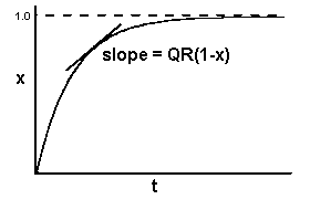
dx/dt = QR(1-x)
Graphically we see an epidemic that starts out looking linear, but as x approaches 1, the slope decreases to zero.
In the polycyclic model we make a similar adjustment:
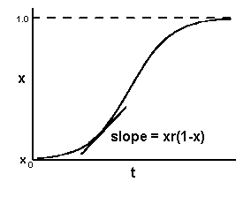
dx/dt = xr(1-x)
This model starts out approximately exponential, but its slope also decreases and approaches zero as xincreases and approaches one. The result is a sigmoid-shaped curve:
In reality, it is rare that disease incidence or severity exceeds 50%, and when it does, the disease progress curve is usually not quite sigmoid. For a discussion of other models of disease progress, see Neher and Campbell, 1992 and Gilligan, 2002.
Estimating Model Parameters
Transformations
To apply our models to real epidemics, we would like to come up with numerical values for their parameters (Rin the monocyclic model and x0 and r in the polycyclic model). To estimate the parameters, we observe the epidemic, measure x at several times during the epidemic, and then plot x versus t. The difficulty comes in trying to fit nonlinear models to the data sets. It is far easier to transform the x's to get a linear model that can be fit with simple linear regression.
The monocyclic model
In the case of the monocyclic model, if the observed x's are transformed to the natural logarithm of 1/(1-x), and these transformed values are plotted against t, we will get a straight line with a slope equal to QR.
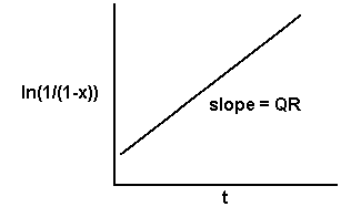
Then with an independent estimate of the initial inoculum, Q,we can calculate R.
The polycyclic model
If the observed x's in a polycyclic epidemic are transformed to the natural logarithm of x/(1-x), and the transformed values are plotted against t, the result will be a straight line witha slope equal to r and an intercept equal to the natural log of x0/(1-x0).
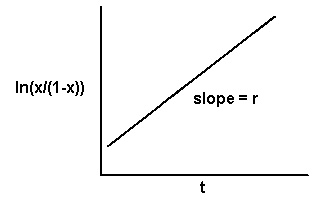
In fitting models to observed data, it is important to select the model based on the known biology of the pathogen rather than simply on the shape of the curve. Likewise, one must not attempt to make inferences about the biology of the pathogen based on the shape of the curve and which model gives the "best fit" of the data. There is random variability in each observation, and in the transformed models the data points on the ends of the line have undue weight in determining the fit to the model. It is quite possible to have a data set that fits both the monocyclic and polycyclic models equally well or to have a data set from a known monocyclic epidemic that gives a better fit to a polycyclic model and vice versa.
Some examples
Example 1, a monocyclic epidemic: Flax wilt is caused by the fungus Fusarium oxysporum f. sp. lini. Chlamydospores of the fungus persist for several years in the soil, and when flax is planted in an infested field, the young plants are infected through the roots. An extensive soil survey was made of a heavily infested field, and it was found to contain an average of 57 colony-forming units per gram of soil. When a susceptible flax cultivar was planted in this field, the percent of plants showing wilt symptoms increased with time as follows:
| Days After |
% Plants |
| Planting |
Infected |
| 10 |
18 |
| 20 |
56 |
| 30 |
82 |
| 40 |
91 |
| 50 |
96 |
| 60 |
98 |
In a plot of disease progress, note how the percent infection asymptotically approaches 100 percent.
[Click for larger graph]
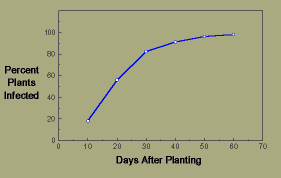
Flax wilt disease progress
To estimate the product, QR, we first have to convert percent infection to the proportion, x, and then using the transformation appropriate for the monocyclic model, calculate ln(1/(1-x)).
| t |
x |
ln(1/(1-x)) |
| 10 |
.18 |
0.198 |
| 20 |
.56 |
0.821 |
| 30 |
.82 |
1.71 |
| 40 |
.91 |
2.41 |
| 50 |
.96 |
3.22 |
| 60 |
.98 |
3.91 |
From a plot of ln(1/(1-x)) versus t, we can fit a straight line to the data points using least squares regression.
[Click for larger graph]
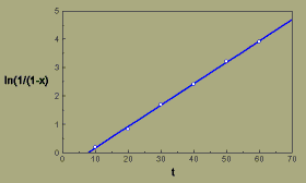
Flax wilt, multiple hit transformation
The slope of the line estimated by the regression equation is 0.076, which is the value of QR. Therefore,
R = 0.076/57 = 0.0013/CFU/Day.
Example 2, a polycyclic epidemic: Halo blight of beans is caused by the bacterium Pseudomonas syringae pv. phaseolicola. The major source of initial inoculum is infected seeds that when planted give rise to plants with lesions on the primary leaves. Bacteria produced in these lesions are splash dispersed to adjacent healthy plants. New lesions can themselves produce secondary inoculum within about 4-5 days. Under conditions moderately favorable for disease development, the following observations were made of disease progress:
Days After
Planting |
% Plants
Infected |
| 10 |
1 |
| 20 |
4 |
| 30 |
15 |
| 40 |
31 |
| 50 |
65 |
| 60 |
88 |
| 70 |
94 |
Disease progress shows the sigmoid-shaped curve characteristic of a polycyclic epidemic.
[Click for larger graph]
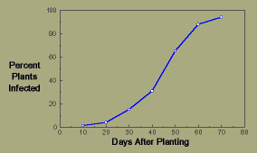
Halo blight disease progress
As with the previous epidemic, we have to convert the percents to proportions (x), but this time the transformation that we use is ln(x/(1-x)).
| t
|
x
|
ln(x/(1-x)) |
| 10 |
.01 |
-4.60 |
| 20 |
.04 |
-3.18 |
| 30 |
.15 |
-1.75 |
| 40 |
.31 |
-0.80 |
| 50 |
.65 |
0.62 |
| 60 |
.88 |
1.99 |
| 70 |
.94 |
2.75 |
By plotting ln(x/(1-x)), sometimes called the logits of x, versus t, we can fit a straight line to the data points with least squares regression.
[Click for larger graph]
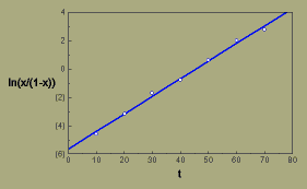
Halo blight, logistic transformation
The regression gives us a slope of 0.124/day, which is our estimate of the apparent infection rate, r.
Obviously the more data points that we have, particularly if they are relatively evenly distributed on both sides of 50% infection, the better estimate we will have of the apparent infection rate. However, it is possible to make a rough estimate of the apparent infection rate with just two data points. Let us suppose for a moment that instead of observations every ten days during the epidemic, we only made two observations, one early (day 10) and one late (day 70). How might we estimate the apparent infection rate? In this case we would be using only the first and the final points in the plot of the transformed data above and calculating the slope as the rise over the run:
r = (ln(0.94/(1.0-0.94)) - ln(0.01/1.0-0.01))) / (70 - 10)
= (2.75 + 4.60) / 60
= 0.123/day
Practical Uses of Epidemiological Models
Example 1: Suppose that in the flax wilt example we surveyed an adjacent field and found a level of initial inoculum that was 1% of that in the field showing severe wilt symptoms. What incidence of infection would we expect in this field at the end of the season (60 days)? To simplify the calculations, let us assume that the final incidence will be so low that we can ignore the correction for healthy plants remaining and use the simple linear model. In our example we averaged of 57 colony-forming units per gram of soil, so 1% of that would be 0.57 CFU. We calculated R to be 0.0013/CFU/Day, and therefore the proportion of plants infected after 60 days would be:
x = QRt = (0.57)(0.0013)(60)
= 0.044 or about 4%
Example 2: Suppose that in the halo blight example we wanted to estimate what incidence of seed infection would be the maximum tolerable to keep the final incidence of disease below 25%. We will assume a 90-day season, and again because the final incidence is low, we will ignore the logistic correction and use the simple exponential model:

Substituting 0.25 for x, our estimated 0.124/Day for r, and 90 Days for t, we get:
0.25 = x0 exp((0.124)(90))
0.25 = x0 exp(11.16)
x0 = 0.25/70263 = 0.0000036
This calculates to an initial disease incidence of about one plant in 280,000.
Next: Plant Disease Management Strategies
