One of the many applications of simulation modeling in plant disease epidemiology pertains to host plant resistance, which can be seen as a major, and possibly the most important, contribution of botanical epidemiologists to sustainable agriculture (Johnson, 1984). The case of partial resistance deserves specific attention, because it illustrates very well the connection between experimental research and conceptual thinking encapsulated in modeling work. Studies on host plant resistance provide numerous examples of the research loop: induction - testing - deduction. This section will show that simulation modeling can make this research loop forward-looking, and enable research to consider the outcomes of choices. Recent advances in molecular plant pathology (Poland et al., 2009) actually now offer a bridge between epidemiology and molecular pathology through simulation modeling.
The induction phase involves (1) observing, exploring (experimentally), and designing the considered system and its structure (modeling); the testing phase (2) involves the measuring of epidemiological parameters, the (experimental) quantification of the system, that is, of epidemics, model parameterization, model verification, and comparing simulation outputs with field data (modeling); and the deduction phase involves (3) assessing levels of resistance of novel, existing or potential, genetic material. Modeling can thus become a very powerful tool for phenotyping host plant resistance.
The nature of host plant resistances
Host plant resistance in plants comes in many forms. Early works (Van der Plank, 1963; Flor, 1946; 1971; Agrios, 2005), from the "host point of view", emphasized horizontal or vertical resistances, and from the "pathogen point of view", emphasized specificity or non-specificity. After decades of research, these clear, almost Manichean, divides have come to be questioned. From the host point of view, the very nature of host plant resistance is now seen as a much more complex phenomenon than initially thought, with many different facets and outcomes. Complete, pathogen-specific, resistance, which was long perceived fragile, because it can, on principle, easily be overcome by pathogen populations under heavy selection pressure, is now seen from a different perspective; some of these complete resistance genes do appear to confer durable resistance (Poland et al., 2009). In other words, there are different types of complete resistance. These different types of complete resistance are thus mirrored by differences in the genetic make-up of pathogen populations. Indeed, durable host plant resistance has been, and still is, the ultimate goal of plant pathologists, geneticists, and breeders alike (e.g., Robinson, 1976; Bonman et al, 1992). The reasons for the central importance of this goal is that durable resistance, a science-based, seed-borne technology, can comparatively be easily deployed, and does not have negative environmental impacts on human and animal health. Durable resistance can also be readily available, especially if carried by inbred (or perennial) varieties, to resource poor farmers, who still represent the bulk of the world farmers' population today.
One often speaks today of qualitative resistance (QLR) and quantitative resistance (QDR). Quantitative (i.e., partial, or incomplete) resistance comes in different shades of grey (Poland et al., 2009). It has been recognized long ago that qualitative resistance may be associated to one locus, and that it can be overcome (e.g., Eversmeyer and Kramer, 2000). This has for instance led to the recent massive epidemic of new strains of wheat stem rust (caused by
Puccinia graminis Ug99) that are virulent on cultivars carrying widely deployed R-genes (Stokstad, 2007). More recently, QLR genes have been shown to vary, some of them providing long-lasting resistance despite the selection pressure they cause (Poland et al., 2009). Recent results suggest that QDR and QLR may in part be actually determined by the same genetic bases, which had long been envisioned (e.g., Parlevliet and Kuiper, 1977). The latter point might perhaps explain why some QLR provide more durable resistance - being associated with QDR.
Simulation modeling offers a critical tool to bridge knowledge and understanding between molecular geneticists, breeders, and plant disease epidemiologists. One main reason is that simulation modeling enables one to 'see' what otherwise could not be monitored at the systems level ― be it plant, field, or region. Another reason is that simulation modeling can provide a very strong tool to help phenotyping genetic materials (e.g., Zadoks, 1977; Rapilly, 1979; Savary et al. 1990; Andrade-Piedra et al., 2005), which perhaps represents the main bottleneck of breeding programs today.
Components of resistance: general definitions and operational definitions
There is a great deal of difference between a general definition and an operational definition (Zadoks, 1972a), which however are sometimes confused. General definitions can be phrased through sentences and refer to concepts. General definitions are open to debate and offer the possibility of sharing among a large number of scientists. Operational definitions, on the other hand, are developed under the premise that the general definition is accepted and are phrased in a practical, often numerical or algebraic form. Operational definitions are thus the practical implementation of the general definitions they correspond to, and thus can be seen as 'recipes', to apply concepts in a specific context. Operational definitions may enter in such detail that they lose the general, conceptual, value of the general definitions they were borne from. The case of components of resistance is one good example of the translation of general definitions to operational ones.
A component of partial resistance (i.e., of quantitative resistance), as a general definition, is one independent element of a chain that contributes to hampering, to some degree, disease progress. If a combination of components of partial resistance affects the disease cycle collectively, epidemics may be suppressed. Considering the classical infection chain (Kranz, 1990), which connects each individual stage of a pathogen's life cycle (which could be seen as a state variable of the disease cycle seen as a system of its own), one should further consider that components of resistance must not overlap, because each of them affect one specific stage of the disease cycle (Zadoks, 1972b).
The latter remark may have important practical applications. In times where phenotyping host plant resistance has become the most difficult part of breeding programs, it may be critical to be able to link a given QTL or gene to a particular component of resistance. Phenotyping for host plant resistance, especially for partial resistance, which has been elusive for so many decades, and might be within reach given the molecular tools available today, could thus remove a bottleneck of many breeding programs, at least for quite a few pathosystems.
Arithmetic operational definitions of components of resistance
Operational definitions for components of partial resistance corresponding to the epidemiological model discussed in the previous chapters have been developed by Zadoks and Parlevliet in a series of publications (Zadoks, 1972b; Parlevliet, 1977; 1979; Parlevliet and Zadoks, 1977). A component of partial resistance is a dimensionless relative resistance coefficient, RR, which varies between 0 and 1:
0 ≤ RR ≤ 1
in which 1 corresponds to the highest level of resistance for this component (which means that no further progress in the disease cycle is made beyond the corresponding stage of the cycle), while 0 corresponds to maximum susceptibility. In other words, when RR = 1, the disease cycle is stopped at the corresponding stage of the disease cycle, and the epidemic halts; if RR = 0, there is full susceptibility, and the pathogen is allowed to pass this stage unhampered.
In the prototype epidemiological model developed so far, we can consider four components of resistance: for infection efficiency (IE): RRIE; for sporulation (SP): RRSP; for latency period duration (LP): RRLP; and for infectious period duration (IP): RRIP.
The previous chapters have shown that while resistance increases with smaller IE, SP, and shorter IP, resistance decreases with shorter LP. Thus, the equations for relative resistances will vary depending on the direction with which decreasing observed values of IE, SP, LP, and IP will be. Operational definitions are meant to use observations, and what is observed by breeders is always relative. Large breeding programs always have a reference. When it comes to partial resistance, one can never be sure to have, within a given field experiment, the highest possible level of resistance. But what is available is the currently lowest level of resistance, a reference for susceptibility, which can be used as a control. In the case of partial resistance, the best practical reference therefore is a susceptible cultivar, c.
Assuming that the cultivar to be tested is denoted x and that the control is denoted c, the operational definitions for components of partial resistances therefore can be written as relative resistance terms (RR), which are functions of x and c:
RRIE(x) = 1 - [IE(x)/IE(c)];
RRSP(x) = 1 - [SP(x)/SP(c)]; and
RRIP(x) = 1 - [IP(x)/IP(c)].
These equations are based on the assumption that a cultivar x will have values of IE, SP, and IP smaller than (or equal to) the susceptible control. Note that, because IE(x) ≤ IE(c), SP(x) ≤ SP(c), and IP(x) ≤ IP(c), all these terms follow the above condition: 0 ≤ RR ≤ 1. This is because, at the highest possible level of observed susceptibility: IE(x) = IE(c), SP(x) = SP(c), and IP(x) = IP(c).
In the case of latency period duration, however, resistance will correspond to higher LP values. Thus a slightly different equation:
RRLP(x) = 1 - [LP(c)/LP(x)].
As indicated earlier, RRIE, RRSP, RRIP, and RRLP are relative resistance terms, each of which corresponding to a unique, non-overlapping, step of the infection chain: therefore, they can be called components of resistance.
The question then arises on how to combine these components, that is, how to express the relative resistance of a host genotype that carries different levels of each of the separate, independent, components of resistance. The
combined relative resistance, RRc, of a variety carrying several components of resistance must meet the following conditions (Zadoks, 1972b; Savary et al., 1990):
a. 0 ≤ RRc ≤ 1;
b. if all the relative resistances (RRi) corresponding to all components (i) are null, then the combined relative resistance (RRc) is null;
c. if any one of the values of the p components is equal to 1, then RRc = 1;
d. if any one of the values of the components is ≠ 0, then RRc ≠ 0.
Such a set of conditions are met by the following equation (Savary et al., 1988):
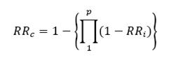
where p is the number of components of resistance involved.
For instance:
if:
RRIE = RRSP = RRIP = RRLP = 1, then
RRc = 1 - {(1 - RRIE) * (1 - RRSP) * (1 - RRIP) * (1 - RRLP)}
= 1 - {(1-1) * (1-1) * (1-1) * (1-1)} = 1 - 0
and: RRc = 1
if:
RRIE = RRSP = RRIP = RRLP = 0, then
RRc = 1 - {(1 - RRIE) * (1 - RRSP) * (1 - RRIP) * (1 - RRLP)} = 1 - 1
and: RRc = 0
if:
RRIE = RRSP = RRIP = RRLP = 0.5, then
RRc = 1 - {(1 - 0.5) * (1 - 0.5) * (1 - 0.5) * (1 - 0.5)} = 1 - {1 - 0.54} = 1 - 0.0625
and: RRc = 0.9375
if one of the components of resistance takes a value of 1 (the disease cycle cannot proceed), for example the first component: RRIE = 1, while RRSP = RRIP = RRLP = 0, then
RRc = 1 - {(1 - 1) * (1 - 0) * (1 - 0) * (1 - 0)} = 1 - {1 - (0 * 1 * 1 * 1)} = 1 - 1
and: RRc = 0
The above equation for calculating RRc on the basis of individual components of resistance is well known to plant pathology. Long ago, G.W. Padwick (1956) used the same equation to assess crop losses in the British colonies, the idea being that what has been lost once cannot be lost twice, thus a product of successive terms.
But this equation can be interpreted in a third way. From a probabilistic stand point, calculating RRc as a product implies that the values taken by each different (non-overlapping) component of resistance reflect independent events. Calculating RRc with the above formula thus assumes that components of resistance, as traits, are governed by independent genetic bases, thus assuming a bridge between phenotypic expression and genetic information. If such were the case, one could envision a straightforward relationship between the phenotypic make-up of a given variety (its field response) and its genetic make-up. Unfortunately components of resistance, however, are often correlated in their phenotypic expression (e.g., Savary et al., 1988) and may have common genetic bases (Poland et al., 2009).
Operational definitions of components of resistance in simulation modeling
The earlier arithmetic equations for components of resistance can be translated for simulation modeling purposes. For a given cultivar x, the epidemiological parameters IE, LP, SP, and IP, can be corrected according to the corresponding components of resistance as follows:
IEcor = IE(x) = IE(c) * (1-RRIE);
SPcor = SP(x) = SP(c) * (1-RRSP);
IPcor = IP(x) = IP(c) * (1-RRIP); and
LPcor = LP(x) = LP(c) / (1-RRLP).
Simulation modeling allows addressing each of the processes of the disease cycle independently and the components of resistance that are attached to them. Over the course of an epidemic, disease cycles may quickly overlap and the effect of a given component of resistance can no longer be detected by the observer. A main advantage of simulation modeling compared to the arithmetic approach outlined above is that it readily enables analyzing the effects of components of resistance on epidemics. In particular, modeling enables disentangling the individual effects of components of resistance in an explicit manner.
Implementing components of resistance in a simulation model
The four components of resistance described above can easily be incorporated in the simplified model developed so far. In a first stage RRIE and RRSP will be addressed, then RRLP, and lastly RRIP.
In the previous chapters, the rate of infection was calculated as:
INFECTION = (DMFR * CORF * InfS) + INOCPRIM,
where INFECTION is the rate of new infections per day (dimension: [N.T-1]), DMFR is our numerical equivalent of Van der Plank's (1963) rate of infection corrected for removals (i.e., the number of new infections per lesion per day [N.N-1.T-1]), CORF is the fraction of sites still available to infection ([N.N-1]), InfS is the current number of infectious sites ([N]), and INOCPRIM is an inflow of infectious propagules ([N.T-1]).
Let us consider DMFR in a little more detail, and say that it consists of the product of two components: first, the inflow of propagules (spores) that may lead to infections, and second, the infection efficiency of these propagules (Zadoks, 1971). Thus:
DMFR = IE * SP, where:
DMFR ≡ [Nlesion.Nlesion-1.T-1];
Botanical epidemiology deals with two interacting populations: that of the plant host, which is represented by sites, and that of pathogen units. Pathogen units may take many forms, but for the sake of simplicity, let us assume that two types of pathogen units are considered here: lesions and propagules. The translations of lesions into propagules, and from propagules into lesions, are complex processes. We cannot address here the extremely diverse range of life cycle strategies plant pathogens have, despite their importance. What is important at this stage is to be are aware of the possibility of these transitions: some lesions produce propagules, and some propagules (sometimes, very few indeed) produce lesions. Thus, speaking of the number of pathogen units, one may use the same dimension: [Nlesion] ≡ [Npropagule].
IE is the number of lesions generated per effective propagule (i.e., effectively coming into contact with the host):
IE ≡ [Nlesion.Npropagule-1] ≡ [Nlesion.Nlesion-1];
and SP is the number of propagules produced per lesion per unit time:
SP ≡ [Npropagule.Nlesion-1.T-1] ≡ [Nlesion.Nlesion-1.T-1].
SP is thus directly linked to InfS, the number of infectious sites, and their ability to produce propagules that may cause new infections, and IE accounts for the efficiency of these propagules to infect. The equation for INFECTION can then be written as:
INFECTION = (IEcor * SPcor) * InfS * CORF + INOCPRIM
with
IEcor = IE(c) * (1-RRIE) = 0.3 * (1-RRIE),
since IE(c) = 0.3 is the infection efficiency of the reference susceptible cultivar, and
SPcor = SP(c) * (1-RRSP) = 1 * (1-RRSP),
since SP(c) = 1 is the term used for the reference susceptible cultivar (i.e., each lesion produces one propagule that potentially may lead to infection at each time step); this also amounts to the equivalency: SP = InfS.
RRLP and RRIP, being delay functions, are handled differently in the model. In the case of the latency period duration, longer LP values correspond to stronger resistance, while it is the opposite in the case of the infectious period. Thus:
LPcor = LP(c) / (1-RRLP) = 6 / (1-RRLP)
since 6 days was the default value for the residence time of lesions in the latent stage. Since this is a residence time, this change is not made on the inflow to the state variable for latent lesions, LatS (which would amount to changing the rate of infection) but to the rate of outflow from the latent stage. Similarly:
IPcor = IP(c) * (1-RRIP) = 10 * (1-RRIP)
since 10 days was the value chosen to represent maximum susceptibility in the previous versions of the model. Again, this change is applied to the outflow from the infectious stage, towards removal.
These changes are shown in the flow diagram of Fig. 6.1, and the program listing is provided in Appendix 6.1.
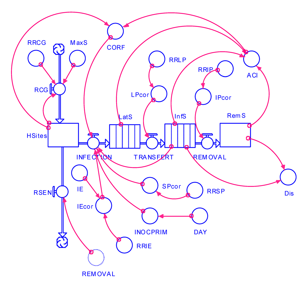
Figure 6.1. Flowchart of an epidemiological simulation model incorporating components of resistance.
Important remarks
In the above paragraph, we considered DMFR as the product of the inflow of propagules (spores) that may lead to infections by the infection efficiency of (effective) propagules, i.e.: DMFR = IE * SP. This enabled us to incorporate in the model components of resistance for infection efficiency and propagule production.
What is meant here by "propagule production" needs clarification. In the case of an aerially-dispersed pathogen, the classical stages are: "propagule formation", "liberation", "transport", and "deposition" (e.g., Kranz, 1978; Zadoks and Schein, 1979). Equivalents could be determined (and operationally defined; Butt and Royle, 1980) in the case of vector-borne (e.g., Madden et al., 2000) or soil-borne (e.g., Gilligan, 1990) diseases.
Therefore, what we refer to here as "propagule formation" (SP) covers, in an admittedly loose way, several, complex, and concatenated processes of the infection chain. Specifically, for a vector-borne pathogen, SP refers to the number of propagules that have been acquired from a mother lesion, then transmitted and inoculated to a target host site, which may become a daughter lesion.
The very notion of lesion may vary from disease to disease. In some cases, individual root segments or fractions of leaves will do; in others, one will better focus on shoots or fruits; and in many diseases, one should consider entire plants. For instance, in the case of many vector borne diseases, the notion of lesion may be a whole plant or a tree (Savary et al. 2012).
Again, this brings us back to the critical issue of choosing the right state variables of a system and its limits, which were introduced in Chapter 1.
Let us focus a little more on aerially dispersed diseases. In this case, SP refers to those propagules that have been produced, liberated, transported, and deposited on a host site (whether infected or not). In the case of many aerially dispersed pathogens, the corresponding lesion often is a fragment of host tissue (e.g., a spot on leaf or fruit) or a fragment of host unit (e.g., a shoot, or a branch; Savary et al. 2012). Thus, SP is a shortcut, and refers to the number of propagules that are effectively made available for potential infection, per unit time and per "mother" lesion.
Still, much detail could be experimentally measured and accounted for in a mechanistic model. In the case of peanut rust, for instance (Savary et al., 1990), the above processes, and others, were taken into account through relative rates of:
- liberation (which depends on relative humidity and the occurrence of rainfall),
- exhaustion of uredosori after a dispersal event (which depends on relative humidity and the occurrence of rainfall),
- deposition (which depends on whether the canopy is dry or not),
- survival and death of spores after they have been deposited (a function of time since liberation),
- spore leaching from pustules in the canopy if rainfall exceeds a given threshold.
Whether such details truly are necessary must be pondered. This was not incorporated in this modeling exercise.
Simulated effects of components of resistance
A first question one may want to address is whether and to what extent the combinations of components of resistance may suppress epidemics. In a first set of runs all the components of resistance were made equal (RRi), and three runs were performed: RRi = 0 (no partial resistance), RRi = 0.1 and RRi = 0.2. The results are shown in Fig. 6.2, with very strong effects, even when all components of resistance are set to 0.1.
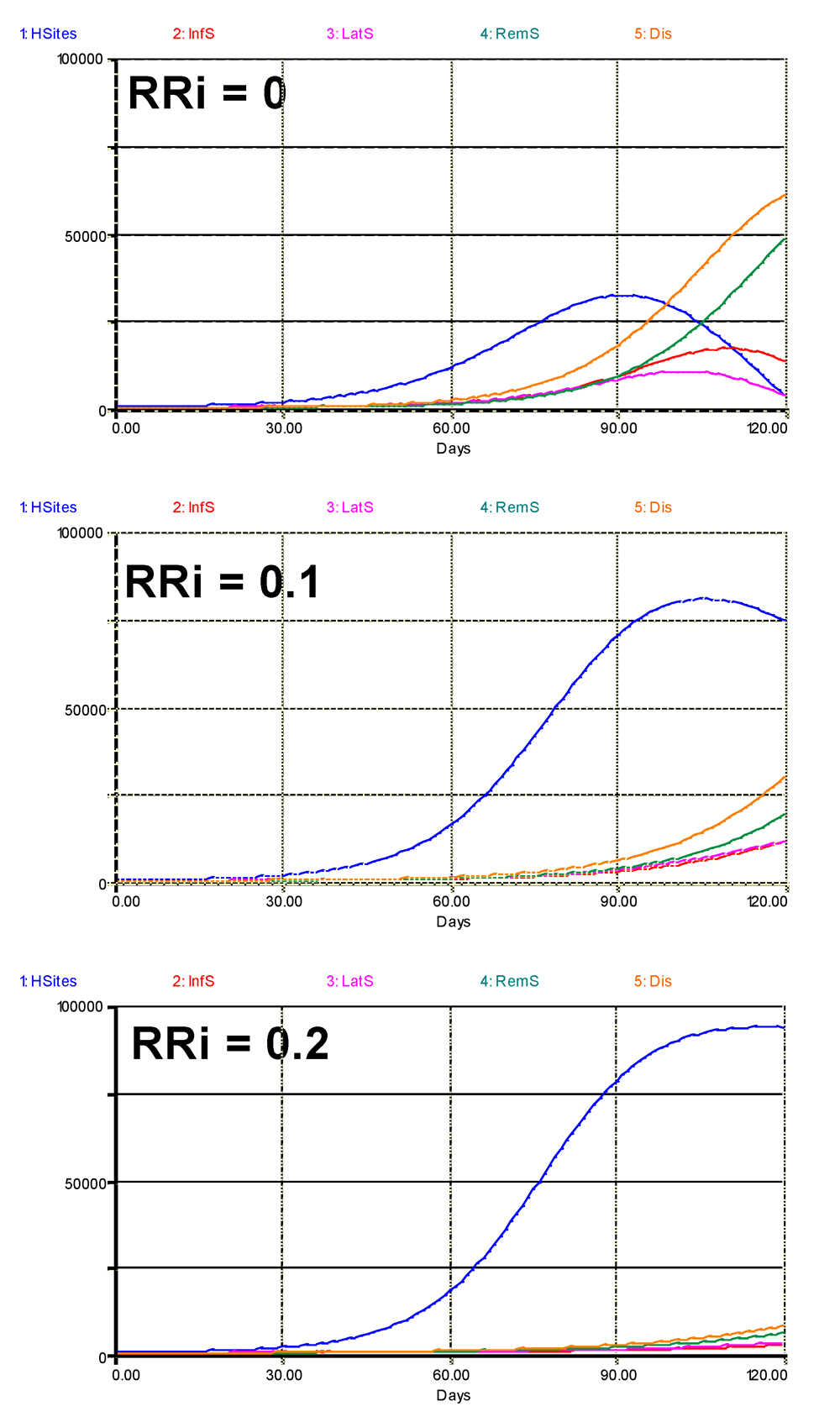
Figure 6.2. Overall simulated effects of increasing levels of components of partial resistance, where RRIE = RRSP = RRLP = RRIP = RRi are set to three values, 0, 0.1, and 0.2. 1: healthy sites; 2: infectious sites; 3: latent sites; 4: sites removed from the epidemiological process; 5: accumulated visibly diseased sites (infectious and removed). Horizontal axis: time (days); vertical axis: numbers of sites.
A second question concerns which component of resistance has the strongest suppressive effect, given the model structure we developed, and its underlying hypotheses. The outputs of such analysis are shown in Fig. 6.3, where each component was given a value of 0.2 in turn. The first run (top left) is identical to the simulation shown at the top of Fig. 6.2, where all components of resistance are null. The second run pertains to RRIE or RRSP, since any partial resistance on these two components have the same bearing within the chosen model structure. In that case, the terminal level of disease is not strongly reduced, but the rate of the epidemic is strongly reduced, with a disease progress curve becoming exponential, while it is logistic in the absence of resistance. The latent, infectious, and removed progress curves are also strongly reduced in their rates. A strong increase in crop growth also occurs. The effects of a partial resistance in the latent (RRLP) or infectious (RRIP) stages have graphically similar effects. Comparing the effects of an increased RRLP and RRIP, however, indicates a strong reduction in the terminal numbers of latent and infectious sites. If the simulation run were longer (e.g., 150 instead of 120 days; not shown), an increased RRLP leads to a near-complete exhaustion of sites, except for the post-infectious (removed) ones, and a collapse of the healthy sites; whereas an increased RRIP in effect delays the exhaustion of latent and infectious sites and, surprisingly, enables a renewed increase of healthy sites in the end of the run.
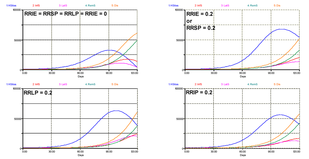
Figure 6.3. Simulated effects of individual components of resistance. 1: healthy sites; 2: infectious sites; 3: latent sites; 4: sites removed from the epidemiological process; 5: accumulated visibly diseased sites (infectious and removed). Horizontal axis: time (days); vertical axis: numbers of sites.
Dealing with pathogen diversity
Pathogen diversity is a fact, which accounts for, among many other things, resistance genes being overcome. For a long time, the process of resistance genes being overcome was considered to apply to qualitative resistance only: a qualitative (complete) resistance exerts such a selection pressure that isolates of the pathogens that can overcome the qualitative resistance emerge and replace the former pathogen genotypes. Could this be so in the case of partial resistance? In the beginning of this chapter, a brief overview of the diversity of resistances was given. One may consider that such a diversity also exists among pathogens (which may vary in terms of virulence or avirulence, or in degrees of aggressiveness), as well as among the mechanisms through which resistances may be overcome.
Let us consider a simplified case where only two isolates of the same pathogen occur.
Isolate 1 has the following characteristics:
- it represents 95 of the 100 initial infections at epidemic onset (t = 20 days);
- the cultivar variety has a low level of partial resistance to isolate 1, with RRIE = RRSP = RRLP = RRIP = 0.1;
while isolate 2 has the corresponding characteristics:
- it represents only 5 of the 100 initial infections at epidemic onset;
- the cultivated variety has no partial resistance to isolate 2.
The results of the simulations are shown in Fig. 6.4. In terms of proportion of isolates (expressed as 'visibly' diseased sites), the dynamics of isolate 2 of course is delayed. Nevertheless, with a much stronger slope, the final number of sites diseased with isolate 2 is higher. This particular output illustrates again one of the major strengths of modeling; that is, its ability to 'see' disease progress, whereas, of course, lesions caused by different isolates cannot be visually distinguished.

Figure 6.4. Dual dynamics of two isolates with differing adaptations to partial resistance. Note that the dynamics of isolates include the variation of the rate of infection over time. 1: healthy sites; 2: infectious sites; 3: latent sites; 4: sites removed from the epidemiological process; 5: accumulated visibly diseased sites (infectious and removed). Horizontal axis: time (days); vertical axis: numbers of sites.
Crop growth is affected as in the previous outputs, with a sharp decline at the end of the run, while the removed sites accumulate.
The dynamics of the two isolates are quite different. The outputs at the bottom of Fig. 6.4 show the value of the rates of infection (INFECTION) of both isolates. While that of isolate 1 is initially high, it rapidly slows down, and tapers off. By contrast, the rate of infection of isolate 2 is initially very low, then increases sharply to a much higher maximum, and declines too, but only at the end of the simulation, as the dual epidemic is running out of healthy sites. Similarly, the numbers of latent and infectious sites are much higher for isolate 1 than isolate 2 at the onset of the epidemic. If another simulation were executed using the final values of this run, isolate 1 would be displaced by isolate 2, and the partial resistance would be overcome. Over successive seasons (or if the crop cycle were longer), this would lead to a population displacement, where the more aggressive strain of the pathogen would eventually dominate.
Perspectives and challenges
The possibility of implementing integrative biology at the system level would represent a major scientific milestone. Progress in molecular biology is now such that never has this possibility been so real. Simulation modeling could play a key role in such advances, especially to breed durable host plant resistances. New genomic platforms in crop species, such as a nested association mapping populations, are providing unprecedented tools to identify quantitative trait loci (QTLs; Poland et al., 2009). Linking field ("phenotyping") data to molecular information through simulation modeling might become a reality (Yin et al., 2004), bridging several levels of integrations of life (from the gene to the individual plant, and to the plant population; de Wit and Goudriaan, 1978). This is fraught with difficulties, of course, but worth considering, for instance, through stepwise integration of sub-models. Difficulties might not lie only in the modeling, but in the use of suitable, reliable phenotyping data too (Parlevliet, 1979).
Challenges are also related to the nature of the host plant, or the pathosystem:
- some host crops may be more difficult to handle than others, making breeding programs more difficult;
- because of their seeds: working on cereals is far easier than on tuber crops, for instance
- because of their life cycle ― the life cycle of a cassava crop lies between 12 to 18 months (with no sexual reproduction occurring in the field); perennials are very difficult to address, not only because of their long life cycles, but also their complex genetic make-ups;
- partial resistance can be very hard to address in some pathosystems. Soil-borne and vector-borne pathogens were mentioned at the beginning of this chapter, thus difficulties arise from
- the complexity of the underlying system (vector-borne diseases); or difficulties in observing and measuring processes (soil-borne diseases), or both;
- and, ironically, some pathosystems are hard to address because they involve such a simple life-cycle of the pathogen. Such is the case of blights caused by, e.g.,
Rhizoctonia solani.
- the above problem may be compounded by the fact that epidemics are so strongly dependent on crop growth (they actually can be termed 'canopy-borne', even if the inoculum is not). This leads to the complex task of partitioning the effects of QTLs that affect plant habit, of QTLs that may influence partial resistance, or both (Srinivasachary et al., 2011).
Simulations
The STELLA® model provided with this chapter (EPIDEMRES.STM) will allow you to explore the model structure and equations, and run the model with varying values of components of resistance, and see their effects on simulated epidemics.
Summary
- Simulation models can be used to address host plant resistance, especially quantitative host plant resistance.
- Simulation modeling can thus become a very powerful tool to phenotyping host plant resistance, because it allows one to track, over time, processes that cannot be seen, and can be linked with current advances in molecular breeding.
- A component of partial resistance (i.e., of quantitative resistance) is one independent element of a chain that contributes to suppressing, to some degree, disease progress.
- A component of partial resistance is equivalent to a dimensionless relative resistance coefficient, RR, which varies between 0 and 1: 0 ≤ RR ≤ 1.
- Components of partial (quantitative) resistance can be defined, for instance for infection efficiency, spore production, infectious period and latency period: RRIE, RRSP, RRIP, and RRLP.
- Conversely, a relative (quantitative) resistance, RRc, of a variety carrying several components of resistance can be calculated.
- These components can be implemented in the simulation model developed so far, and the effects of each component, alone or in combination, can be assessed.
- Pathogen diversity, in terms of varying levels of aggressiveness, can be addressed as well. An example of a variety with components of resistance confronted with two isolates differing in aggressiveness is given, where quantitative (partial) resistance is overcome, leading to population displacement by a more aggressive pathogen strain.
- A STELLA® model is provided, allowing users to run the model with varying values of components of resistance, and see their effects on simulated epidemics.
References
Agrios, G.N. 2005. Plant Pathology, Fifth Edition. Elsevier Academic Press, Burlington, MA, USA.
Andrade-Piedra, J. L., Hijmans, R. J., Forbes, G. A., Fry, W. E., and Nelson, R. J. 2005. Simulation of potato late blight in the Andes. I: Modification and parameterization of the LATEBLIGHT model. Phytopathology 95:1191-1199.
Bonman, J.M., Khush, G.S., and Nelson, R.J. 1992. Breeding for resistance to pests. Annual Review of Phytopathology 30:507-528.
Butt, D. J., and Royle, D. J. 1980. The importance of terms and definitions for a conceptually unified epidemiology. Pages 29-45 In: Comparative Epidemiology. A Tool for Better Disease Management. Palti, J. and Kranz, J. eds. Pudoc, Wageningen.
de Wit, C.T., and Goudriaan, J.G. 1978. Simulation of Ecological Processes. Pudoc, Wageningen, 175p.
Eversmeyer, M.G., and Kramer, C.L. 2000. Epidemiology of wheat leaf and stem rust in the central great plains of the USA. Annual Review of Phytopathology 38:491-513.
Flor, H.H. 1946. Genetics of pathogenicity in
Melampsora lini. Journal of Agricultural Research 73:335-357.
Flor, H.H. 1971. Current status of the gene-for-gene concept. Annual Review of Phytopathology 9:275-296.
Gilligan, C. A. 1990. Mathematical modeling and analysis of soilborne pathogens. Pages 96-142 In: Epidemics of Plant Diseases, Second Edition J. Kranz ed. Springer-Verlag, Berlin.
Johnson, R. 1984. A critical analysis of durable resistance. Annual Review of Phytopathology 22:309-330.
Kranz, J. 1978. Comparative anatomy of epidemics. Pages 33-62 In: Plant Disease. An Advanced Treatise, Vol. IV. J.G. Horsfall and E.B. Cowling, eds. Academic Press, New York.
Kranz, J. 1990. Epidemics, their mathematical analysis and modeling: an introduction. Pages 1-11 In: Epidemics of Plant Diseases. Second Edition. J. Kranz, ed. Springer Verlag, Berlin.
Madden, L. V., Jeger, M. J., and Van den Bosch, F. 2000. A theoretical assessment of the effects of vector-virus transmission mechanism on plant virus epidemics. Phytopathology 90:576-594.
Padwick, G.W. 1956. Losses caused by plant diseases in the tropics. Comm. Mycological Inst. Kew, Surrey, Phytopath. Papers N°1, 60 p.
Parlevliet, J. E., and Kuiper, H. J. 1977. Resistance of some barley cultivars to leaf rust,
Puccinia hordei. Polygenic partial resistance hidden by monogenic hypersensitivity. Neth. J. Pl. Pathol. 83:85-89.
Parlevliet, J. E. 1977. Plant pathosystems: an attempt to elucidate horizontal resistance. Euphytica 26:553-556.
Parlevliet, J. E. 1979. Components of resistance that reduce the rate of disease epidemic development. Annual Review of Phytopathology 17:203-232.
Parlevliet, J. E., and Zadoks, J. C., 1977. The integrated concept of disease resistance: a new view including horizontal and vertical resistance in plants. Euphytica 26:5-21.
Poland, J. A., Balint-Kurti, P. J, Wisser, R. A., Pratt, R. C., and Nelson, R. J. 2009. Shades of gray: the world of quantitative disease resistance. Trends in Plant Science. 14:21-29.
Rapilly, F. 1979. Simulation d'une épidémie de
Septoria nodorum Berk. sur blé. Etude des possibilités de résistance horizontale. Bull OEPP 8:243-250.
Robinson, R. 1976. Plant Pathosystems. Springer Verlag, Berlin, Heidelberg, New York, 184p.
Savary, S., Noirot, M., Bosc, J.P., and Zadoks, J.C. 1988. Peanut rust in West Africa: a new component in multiple pathosystem. Plant Dis. 78: 1001-1009.
Savary, S., De Jong, P.D., Rabbinge, R., and Zadoks, J.C. 1990. Dynamic simulation of groundnut rust, a preliminary model. Agricultural Systems 32: 113-141.
Savary, S., Nelson, A., Willocquet, L., Pangga, I., and Aunario, J. 2012. Modelling and mapping potential epidemics of rice diseases globally. Crop Protection 34: 6-17.
Srinivasachary, Willocquet, L., and Savary, S. 2011. Resistance to rice sheath blight (Rhizoctonia solani Kuhn) [teleomorph:
Thanatephorus cucumeris (A.B. Frank) Donk.] disease: current status and perspectives. Euphytica 178:1-22.
Stokstad, E. 2007. Deadly wheat fungus threatens world’s breadbaskets. Science 315, 1786–1787
Van der Plank, J.E. 1963. Plant Diseases. Epidemics and Control. Academic Press, New York.
Yin, X., Struik, P. C., and Kropff, M. J. 2004. Role of crop physiology in predicting gene-to-phenotype relationships. Trends in Plant Science 9:426-432.
Zadoks, J. C. 1971. Systems analysis and the dynamics of epidemics. Phytopathology 61:600-610.
Zadoks, J. C. 1972a. Methodology in epidemiological research. Annual Review of Phytopathology 10:253-276.
Zadoks, J. C. 1972b. Modern concepts in disease resistance in cereals. Pages 89-98 In: The Way Ahead in Plant Breeding. F.A.G.H Lupton,, G. Jenkins, and R. Johnson, eds. Proc. 6th Cong. Eucarpia. Cambridge, 89-98.
Zadoks, J.C. 1977. Simulation models of epidemics and their possible use in the study of disease resistance. Pages 109-118 In: Induced Mutations Against Plant Diseases. IAEA, Ed. Vienna.
Zadoks, J. C., and Schein, R. D. 1979. Epidemiology and Plant Disease Management. Oxford University Press, New York. 427p.
Zadoks, J. C., and Van Leur, J. A. J. 1983. Durable resistance and host-pathogen-environment interaction. Pages 125-140 In: Durable Resistance in Crops. F. Lamberti, J. M. Waller, and N. A. Van der Graaff, eds. Plenum Publishing Corporation, New York.
Exercises and questions
Questions
1. A component of resistance
- can take values above 1
- can affect different processes of the monocycle
- affects only one process of the monocycle
- decreases when its effect on the monocycle processes increases
2. The different components of resistance
- may have different effects on the simulated epidemics
- have the same effects on the simulated epidemics
- have an additive effect when combined
- have a more than additive effect on epidemics when combined
3. Do components of resistance have a direct effect on yield?
Answers
1. c: affects only one process of the monocycle.
2. a: may have different effects on the simulated epidemics, and d: have a more than additive effect on epidemics when combined.
3. No. Components of resistance slow epidemics down. They may have, through this reduction of disease, a strong effect on yield in some cases.
Appendix 6.1. Program listing of EPIDEMRES
HSites(t) = HSites(t - dt) + (RCG - INFECTION - RSEN) * dt
INIT HSites = 100
INFLOWS:
RCG = RRCG*HSites*(1-(HSites/MaxS))
OUTFLOWS:
INFECTION = ( (IEcor*SPcor) * CORF * InfS) + INOCPRIM
RSEN = REMOVAL
InfS(t) = InfS(t - dt) + (TRANSFERT - REMOVAL) * dt
INIT InfS = 0,0,0,0,0,0,0,0,0,0
TRANSIT TIME = varies
INFLOW LIMIT = INF
CAPACITY = INF
INFLOWS:
TRANSFERT = CONVEYOR OUTFLOW
TRANSIT TIME = 6*LPcor
OUTFLOWS:
REMOVAL = CONVEYOR OUTFLOW
TRANSIT TIME = 10*IPcor
LatS(t) = LatS(t - dt) + (INFECTION - TRANSFERT) * dt
INIT LatS = 0,0,0,0,0,0
TRANSIT TIME = varies
INFLOW LIMIT = INF
CAPACITY = INF
INFLOWS:
INFECTION = ( (IEcor*SPcor) * CORF * InfS) + INOCPRIM
OUTFLOWS:
TRANSFERT = CONVEYOR OUTFLOW
TRANSIT TIME = 6*LPcor
RemS(t) = RemS(t - dt) + (REMOVAL) * dt
INIT RemS = 0
INFLOWS:
REMOVAL = CONVEYOR OUTFLOW
TRANSIT TIME = 10*IPcor
ACI = LatS+InfS+RemS
CORF = 1-(ACI/(ACI+HSites))
DAY = TIME
Dis = InfS+RemS
IE = 0.3
IEcor = IE*(1-RRIE)
INOCPRIM = IF (DAY=20) THEN 100 ELSE 0
IPcor = 1*(1-RRIP)
LPcor = 1/(1-RRLP)
MaxS = 100000
RRCG = 0.1
RRIE = 0
RRIP = 0
RRLP = 0
RRSP = 0
SPcor = 1-RRSP

