A few definitions
A
system is a simplified representation of reality. "System" is a common word, often used with loose meaning. Whereas in the real world, a "system" may seem at times an endless series of connected elements, we refer here to a system as (1) a series of selected, chosen elements (this is a first simplification, and thus an implicit assumption), with (2) specified boundaries (a second simplification and implicit assumption), and (3) pre-determined time characteristics (with a third simplification and implicit assumption).
These simplifications over space and time are important: they require pondering, and thus, expertise on the reality at hand. A 'simple' system could for instance be a nearby coffee shop. This coffee shop has customers who place orders and staff who process them. There may be at times very few customers, whereas at others, the place is very busy (say, because the coffee shop is just nearby the University, and has free wi-fi, which the students use while enjoying a coffee and chat with their friends). So, for the customers, and the staff too, time is not neutral. It is then useful to look at our coffee-shop-system over a series of sections of time (time steps) that make a day. Perhaps an appropriate time step of one hour is adequate: it is more than enough to encapsulate long hours when little really happens, but is just enough to capture events at peak time. So much, though, may happen in one hour over a cup of coffee, when the place is busy, people meet, many orders are placed, many messages received. Perhaps, a time step of 30 minutes, or even 15 minutes might then be better. So, although many near-empty 15-minute segments might be a waste of computing time, and lead to outputs that may be boring for some parts of the day, these might ensure that important events are not lost at peak time. Yet - so many things may still happen over a period of 15 minutes. Might a time step of 5 minutes be safer? This is obviously not an easy question.
At any rate, a decision must be made, and it is up to the modeler to make it. Each system, such as the coffee-shop-system, has a
time constant, which we can simply define for the time being as the delay over which the system may strongly change, or, in systems analysis phrasing: over which the
state of the system may change. One way to empirically choose a time constant is based on experience and knowledge of the system at hand. Note that in the coffee-shop-system, not all the elements are enclosed within the coffee shop itself, which are important for the coffee-shop-system: for instance, it has free wi-fi. We therefore can call it a semi-open system. Biological systems, phytopathological systems in particular, are
semi-open: they receive and transmit information, components, biomass, or energy from and to their environment.
A
model is a computer program that describes the mechanics of the considered system. The encoding of a model can be made in many ways. Here, we use the STELLA® program, which enables us to focus only on components of a system, the system's structure, relationships among components, and the modeled system's behavior, rather than on the code of the program itself. Here, we refer to dynamic simulation models. At each time step, the status of the system changes: in the coffee-shop-system, customers come and go, orders are placed, coffee is drunk, receipts are paid, messages are received, news is shared, sometimes coffee is spilled on computers. At each time step, the model updates the status of the system, and is set ready to account for the events of the following time step on the basis of the new status it just has acquired.
A simulation, simply, is the execution of a model. This requires the further definition of the initial conditions of the system under consideration, and specified values of parameters. Again, this implies expertise on the system at hand. In the coffee-shop-system, one has to decide a few things. When in the day does the modeling start? How many customers and staff are already there at that time? How much money does the cashier have then? What are the prices of the different kinds of coffee? What are the rates of inflow and outflow of customers (and what determines it)? What is the rate of inflow of messages? The modeler, simply, has to set the scene, and decide a few rules. These may be made simple in the beginning.
A preliminary warning remark
The beginning of the previous paragraph started with three elements of simplification regarding the components of a system, the boundary within which a system operates, and the time characteristics of the system under consideration. As in other branches of science, these simplifications are made in order to make the problem tractable. Before we proceed, it is very important to stress that, while science progresses through assumptions (and thus simplifications) that are tested and refuted, such simplifications in modeling do correspond to assumptions. One real danger of modeling without revisiting such assumptions is to make the process of model development, verification, and evaluation an exercise which becomes disconnected from the reality at hand. These simplifications-assumptions are derived from the modeler expertise of a reality, and of hypotheses about components that govern the system's behavior. Not revisiting (and testing) these hypotheses may lead to reductionism, not to the originally intended 'systems approach'.
Analytical and numerical integration: example of the exponential growth
Some basics of calculus are needed for modeling. But this is very little indeed. A classical example is that of exponential growth. If one considers a system in which an organism (say, a bacterium) is provided with unlimited nutrient and conditions that are suitable for its maintenance, growth, and multiplication, then exponential growth is expected to occur. Such a system is of course a very strong simplification of reality, and we shall come back to addressing such simplification in the following chapter.
Nevertheless, let us assume that this system is worthwhile considering for now, and let us denote by
x the number of bacteria, and by
t, the elapsing time. What follows are two approaches to modeling the system. We shall start with an
analytical integration. We then will address the same question with what is called a
numerical integration. This section will end with a brief discussion on the differences between these two approaches.
The analytical integration of the problem could be written as follows. Let us consider a very simple process, whereby a given quantity,
x, increases over time,
t, with a given rate,
r. Let us further assume that
x may vary between an initial value,
x0, and a final value
xf. Conversely, time may vary between a starting time,
t0, and a final time tf, so that one can write:

and

Therefore, one can write that the variation in
x relative to any variation (more precisely, to any infinitely small variation) of time,
dt, is proportional to r and to the value of the currently existing quantity
x:
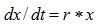
One can note that the quantity
dx/dt is a ratio between the considered quantity and time. If, for example,
x were a distance,
dx/dt would represent the physical speed of an object. In general, these equations refer to some speed of a sort; we shall come back to that point later-on.
This differential equation can be easily handled by 'moving' the
dt term to the right hand-side of the equation, and the
x term to the left hand-side of the equation, so:
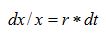
Now that we have all the
xs on the left hand-side, and the time term,
dt, on the right hand-side of the equation, we can use Riemann integrals in order to solve this differential equation, and write:
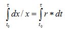
where
t0 and τ denote the initial and final times over which the process is integrated, respectively.
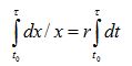
We may assume at this stage that
r, the rate of increase of the quantity under consideration, is constant over the time interval we have chosen
[t0, τ]. With this assumption, r can be extracted from the integral sign of the right hand-side of the equation:
The integration of both sides of the equation can then be done, as:
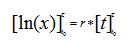
where the
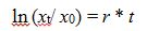
t0 and τ signs on both sides of the brackets indicate, as before, the initial and final times when the integration is made. This translates into:
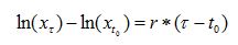
which amounts to:
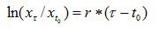
If we simplify the way to write variables as:
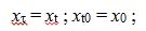
as well as considering that the running time,
τ, can be written as t: τ = t; and if we assume that the initial time is null:
t0 = 0, we can make further simplifications to the equation:
The reverse function of the natural logarithm is an exponential, so that we can write:
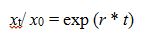
And so, we can write:
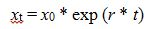
This is the typical exponential growth function, which states that the population of bacteria,
x, increases exponentially, with an initial value of
x0 (when
t = 0,
er*t = e0 = 1), and this growth is infinite.
The numerical integration of the same problem can now be addressed as follows. Let us say that:
- the amount of bacteria is to be denoted by A, the number of bacteria in the system at a given point of time;
- the rate of increase of the bacterial population is denoted RA; and
- the relative rate of increase of the bacterial population, that is, the rate of increase of the bacterial population relative to the amount of bacteria present in the system is denoted RRA.
One notes that, in comparison with the analytical integration, we now have:
A =
x;
RA =
dx/dt, and
RRA =
(dx/dt)/x.
The numerical integration of this problem only involves two lines of code:
A (t + Δt) = A (t) + RA * Δt
RA = RRA * A
The first equation states that at each time step, Δt, the amount A of bacteria at time t, A(t), is incremented by the quantity RA * Δt, and the second, that RA is in turn the product: RRA * A.
These equations can also be summarized by a diagram:
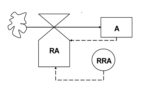
Figure 2.1. A flowchart for exponential growth. The amount of bacteria is denoted A, the rate of bacterial increase is denoted RA at each time step Δt, with a relative (or intrinsic) rate RRA (See also Table 2.2).
One may want to consider if, and to what extent, the principle of the two methods, analytical and numerical integration, differ. Let us come back to the differential equation with which we started:
dx/dt = r * x
If, in this equation, one replaces the infinitely small differences, denoted
d• in bacterium numbers (dx) or in elapsed time (dt), by small variation in bacterium number, Δx, in response to small variation in time, that is, by time step Δt, one would derive:
Let us make Δt approaching infinitely small values, that is, let us consider the limit of the ratio Δx / Δt with Δt becoming infinitely small. One may write:
where
dx / dt is the definition of the derivative of
x over
t. In other words, writing:
is formally incorrect, but one may say that the ratio Δx/ Δt is an approximation of
r * x, if Δt is small enough. One should thus write:
The two approaches therefore are not identical. The formal analytical integration yields the correct result, whereas the numerical integration only provides a numerical estimate. Science of course prefers exact results. Some systems, however, are sufficiently complicated to prevent the derivation of an analytical solution. Should such systems be disregarded for this reason? Numerical integration provides a means to produce approximate solutions. For instance, in the above example, the analytical solution was derived while assuming r constant. This of course very seldom happens, even in highly simplified systems. Numerical integration provides a simple way to address variation over time of parameters such as, in this example,
r. Furthermore, sources of variation other than time can be addressed as well. This will be addressed in the next chapter.
Numerical integration also provides other, quite important, advantages including: (1) means to easily explore the behavior of a system, and (2) means to easily develop, convey, and share model structures and their implications, as we shall try to show.
As pointed out in the first section of this chapter, one must bear in mind elements pertaining to (1) the implicit assumptions-simplifications that form the basis of a model structure, (2) the need for expertise when time steps, systems limits, and systems components are chosen, and (3) the necessity to suitably assess simulation model outputs. Such precautions are needed irrespective of the modeling approach chosen.
Forrester's symbols and syntax
Table 2.1 provides a summary of the symbols Jay Forrester (1961) created, which were used previously in Fig. 2.1 and which will be used throughout the module.
Table 2.1. List of symbols for simulation modeling. After Forrester (1961).
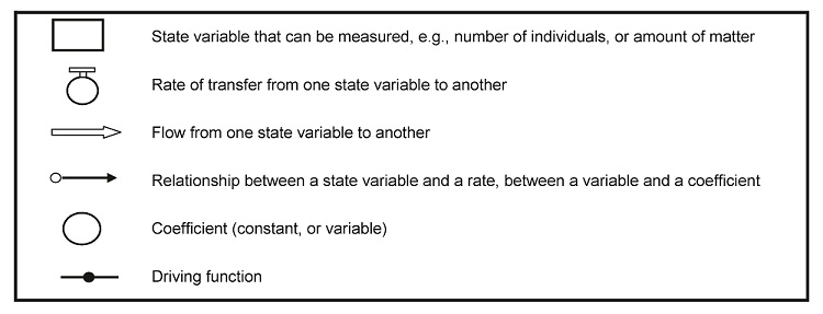
The first symbol is a rectangle, representing a
state variable. State variables characterize a system's status, and are continuously varying in the system. In the above example, the state variable is A, or the number of bacteria. Surprisingly enough, the choice of state variables is critical, and also reflects the interests of the modeler. In the virtual coffee-shop system of the former section, several choices could be made. For instance, a specialist in population dynamics (or professors concerned by attendance in class) would probably choose state variables which express numbers of customers (i.e., which have 'numbers' as dimension, as discussed below); an economist would perhaps choose state variables expressing money exchanged; an information theory specialist might choose state variables representing information in its various forms; or a supply-chain expert might consider stocks of coffee in their various stages of consumption. Such choices have implications on the very use of the model, of course, but also may lead to pondering the limits of the system to consider (what is the limit of information? where does the coffee actually come from?), the flows and connections the system involves, as well as its time-constant. While such choices are in the hands of the modeler, a rule of thumb exists: a 'good' mechanistic model is one which has state variables that have correctly been chosen, because the state of the system is described by several state variables (accounting for a series of relevant transitions in one key component of the system, say, the numbers of incoming, waiting, sitting, paying, and leaving customers), and comparatively few parameters.
This last point brings us to what we feel is a critical remark, although many might perceive it as obvious: modeling must have a purpose. One is often tempted to model 'everything', that is, mix up levels of integrations (e.g., the life cycle of an individual lesion, the dynamics of disease on a plant, the dynamics of disease in a canopy or a landscape, as well as the crop losses caused by disease). This is a very dangerous path to take: systems analysis tells us that the behavior of a system at one level of integration depends on processes occurring at the immediately lower level of integration. Limits must be chosen, and objectives set. The choices of the state variables, of the limits of the system, for instance, are important steps to not drifting towards unmanageable complication. Setting such limits also allows focusing on the applications a model may have.
The second symbol is a
valve which controls a flow incoming or leaving a state variable; this symbol is always connected to the very
flow the valve controls, the third symbol of Table 2.1. There can be only one valve, that is, one control, per flow. Flows are represented in solid arrows (Fig. 2.1) or double lines (Table 2.1). They represent the increase, or decrease, of contents of the state variable the flow reaches or leaves. In Fig. 2.1, rate RA controls the inflow of bacteria into the state variable A, the total number of bacteria in the system.
Systems nearly always involve flows other than those pertaining only to the increase or decrease in contents of state variables. These
flows of information are shown in dashed lines (Fig. 2.1) or in simple thin lines (Table 2.1). A flow of information always originates from a coefficient, a (possibly variable) parameter, a driving function, or from a state variable, as in Fig. 2.1.
Coefficients or parameters are shown as circles, as in Fig. 2.1, where RRA represents the relative rate of bacteria increase.
The last symbol introduced by Forrester (Table 2.1) is that for a
driving function: a segment and a dot at its middle. This brings us back to the beginning of this chapter, when dealing with semi-open systems. Driving functions are meant to represent factors that are not included within the set boundaries of the considered system, but nevertheless, influence it from the outside. Examples for driving functions are many: the Earth system does not include the Sun, yet everything that happens on Earth depends on the radiations intercepted by Earth from the Sun, which therefore may be represented by a driving function; or, the purchasing behavior of customers in the coffee-shop-system may depend on the price of the coffee - or on whether examination dates are approaching. Similarly, in Botanical Epidemiology, the behavior of a pathosystem may strongly depend on temperature or rainfall. Driving functions represent variables that are outside the limits of the considered system, and yet may strongly influence it. They also are likely to vary strongly, and the choice of a suitable time step has to take into account these variations. Some programs, such as the STELLA® program, represent driving variables with the same symbol as (variable) parameters, i.e., circles. However, it is important to bear in mind the clear difference between a parameter (within a system) and a driving function (outside its boundaries).
Dimensions
Dimensions can be represented between brackets. For instance, [L], [T], and [K] stand for length, time, and temperature dimensions, respectively. The speed of an object, for example, would have dimension: [L.T-1], that is, distance per unit of time:
Speed = distance / time
with dimensions:
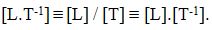
Note that the symbol between L and T-1 does not represent a multiplication sign in the algebraic sense.
An equation such as: RA = RRA * A in the above example entails dimensions.
- A, the size of the bacterial population has for dimension: [bacteria], or: [N];
- RA, the rate of growth of the bacterial population has for dimension: [bacteria.time-1], or in a simplified manner: [N.T-1]; and
- RRA, the rate of growth of the bacterial population relative to the bacterial population size has for dimension: [bacteria.bacteria-1.time-1], or: [N.N-1.T-1]
The dimensionality of the equation:

Since the number dimensions, [N] and [N-1], cancel one another in the right hand side of the dimensionality equation, one thus can see that both sides of the equation for RA have the same dimensions.
Checking the dimensionalities of an equation is one good way to check if the equation itself is correct. Do note, however, that the reverse is incorrect: identical dimensionalities of both sides of an equation are no proof of its correctness (and of course not of its scientific validity). Nevertheless, it is a very convenient way to check for gross mistakes.
Unlike analytical integration, numerical integration therefore deals with dimensions. In particular, the dimension of the state variables that are involved in a model is one key additional decision a modeler must make. In that sense, numerical integration brings us close to the realm of physical sciences, although of course mathematical correctness is required. Choosing, checking, and pondering the dimensions of each of the elements of a model does not cause additional trouble. On the contrary, it provides a critical instrument to control whether the modeling structure is consistent. This is particularly useful when a model involves a number of state variables, rates, parameters, and driving functions. Note that dimensions are related to units. However, a given dimension may correspond to different units, and the latter should of course be consistent across the structure of a model as well.
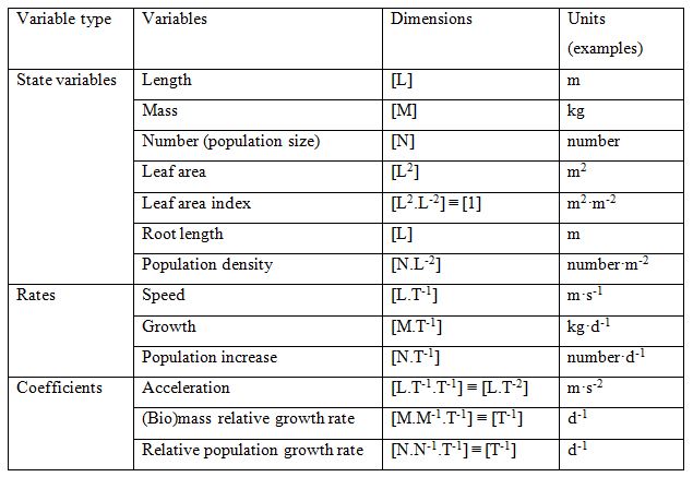
Table 2.2 provides a list of dimensions for state variables, rates, and coefficients. Note, as indicated above, that all the rate variables are actually speeds of some sort, and thus have dimensions: [ _.T-1].
Table 2.2. Dimensions for a set of examples of variables
Time constant and integration step
Let us return to the notion of time constant. As the model runs, a program is executed. Its execution is based on a chosen time step, Δt. At each time step during the running time of the program, each state variable at t + Δt equals the value of the state variable at time t, plus the rate at time t multiplied by Δt. This procedure of numerical integration yields the new values of the state variables.
The time step of the model, Δt, has to be chosen small enough so that the rates do not change notably within Δt. To avoid instability, the time step has to be much smaller than the time constant of the considered system. The time constant of a very simple system such as the bacterial population model considered in this chapter is 1/RRA (note that: 1 / RRA ≡ [T]).
Depending on authors, the time step used should be 1/3rd to 1/5th of the system's time constant. Most systems, however, involve several processes, and therefore, several rates. One may consider that the time constant of such a system is equal to the reverse of the fastest relative rate of change of one of its state variables. The smaller the time constant of a system, the smaller the time step will have to be.
Summary
This chapter introduces the concepts of system, model, and simulation. It also
- introduces the notion of numerical integration, and compares it with analytical integration;
- thus, the notion of time step, its choice, and the concept of time constant are introduced;
- by means of a simple exponential process, the syntax of Forrester to represent systems is introduced;
- and the notion of dimensionality of variables and parameters in a model is explained.
References
Forrester, J.W. 1961. Industrial Dynamics. M.I.T. Press, Cambridge (Mass.).
Penning de Vries, F.W.T., and Van Laar, H.H., eds. 1982. Simulation of Plant Growth and Crop Production. Pudoc, Wageningen.
Rabbinge, R., Ward, S.A., and Van Laar, H.H.,eds. 1989. Simulation and Systems Management in Crop Protection. Pudoc, Wageningen.
Thornley, J.H.M., and France, J. 2007. Mathematical Models in Agriculture. Quantitative Methods for the Plant, Animal, and Ecological Sciences. 2nd Ed. CABi, Wallingford.
de Wit, C.T., and Goudriaan, J.G. 1978. Simulation of Ecological Processes. Pudoc, Wageningen.
Suggested reading
Case, J.T. 2000. An Illustrated Guide to Theoretical Ecology, Oxford University Press, New York.
May, R., and McLean, A. 2007, Theoretical Ecology, Third Edition. Oxford University Press, New York.
Renshaw, E. 1991. Modelling Biological Populations in Space and Time. Cambridge University Press, Cambridge.
Exercises and questions
-
A reasonable time step to simulate the dynamics of the number of books in a library is
a. one second
b. one day
c. one month
d. one year
-
What are reasonable time steps in the coffee shop if one chooses:
a. the number of customers as state variable;
b. the number of coffee cups served as a state variable;
c. the number of incoming and outgoing e-mails as a state variable;
d. the number of employees present at any time in the coffee shop;
e. the amount of money in the cashiers desk at any time.
-
In the modeling of growth of a bacterial population, the rate of growth of the bacterial population, the relative rate of growth of the population, and the number of bacteria are, respectively:
a. a state variable, a rate, and a relative rate;
b. a rate, a relative rate, and a state variable;
c. a relative rate, a rate, and a state variable.
-
A state variable is
a. A rate of change of variable
b. A constant parameter
c. A variable which varies at each time step, depending on inflows and outflows
d. A driving function
-
Numerical integration
a. can be done when parameters vary over time
b. is identical to analytical integration
c. requires mathematical integration
d. does not depend on the integration time step
-
The dimension of speed is
a. [L]
b. [L2]
c. [L.T]
d. [L.T-1]
-
The dimension of the density of bacteria in a suspension is
a. [T-1]
b. [N.L-3]
c. [N.L-2]
d. [L.T-1]
Answers to exercises and questions
- b: one day
- Reasonable time steps are in the range of:
a. for the number of customers: 1 hour;
b. for the number of coffee cups served: 5 minutes;
c. for the number of incoming and outgoing e-mails: 1 minute;
d. for the number of employees present at any time in the coffee shop: 1 hour;
e. for the amount of money in the cashiers desk at any time: 1 hour or 1 day.
- b: a rate, a relative rate, and a state variable.
- c: A variable which varies at each time step, depending on inflows and outflows
- a: can be done when parameters vary over time
- d: [L.T-1]
- b: [N.L-3]

