The analysis and modeling of crop losses is central to plant protection in general, and to plant pathology, in particular: no plant protection scientific reasoning could possibly exist without a measure of crop losses (Chiarappa, 1971; Rabbinge et al., 1989; Savary et al., 2006; Teng, 1987; Zadoks, 1985; Zadoks and Schein, 1979). In many ways, the applied side of phytopathology, as a science, would thus not exist if crop losses to diseases did not occur. Ironically, the information on crop loss is scarce for a number of reasons we shall not elaborate here. Simulation modeling is one approach to complement the existing data, upscale them, and project ourselves in future environmental, social, and technical scenarios. However, this is only possible if reliable field data are available in sufficient number to assess the outputs of models ― simulation outputs cannot be seen
per se as substitute for measured realities. This latter point cannot be addressed here despite its critical importance.
This chapter introduces the effects of pests (pathogens, but also animal pests, and weeds) on crop growth and how they can be incorporated into crop growth simulation models in order to model yield losses. Crop losses, or more specifically yield losses, occur because the physiology of the growing crop is negatively affected by pests in a dynamic way over time as crop both grows (i.e., increases in biomass) and develops (i.e., passes through the different stages of its physiological development). As a necessary first step to achieve the modeling of yield losses we therefore need to introduce concepts that are related to yield levels and damage mechanisms because they represent the conceptual basis of modeling yield losses. The effects of pests on crop growth using the so called "radiation interception - radiation use" (RI-RUE) framework discussed in the previous chapter will then be addressed again. Lastly, the implementation of damage mechanisms into a crop growth model will be presented and illustrated.
Developing simulation models that integrate the dynamic effects of damage mechanisms of injuries caused by pests, and their translation into yield reduction can provide several types of outcomes, both scientific and practical. Note that, because we deal with (physiological) damage mechanisms on the growing crop, the focus is not on the pathogens (pests) themselves, but the injuries each pathogen (pest) may cause: one pathogen (pest) may cause one or several (and quite different) injuries.
Such models enable, for instance, one to gain:
- A better understanding of processes involved in the attrition of crop growth and yield caused by pest injuries; this is the heuristic value of (simple) simulation models. In that case, the system's behavior is analyzed and allows pinpointing knowledge gaps and deriving hypotheses on the system's functioning.
- A better view of the respective importance of pests, with respect to the yield losses they can cause: simulation of yield losses caused by one injury in isolation, versus a combination of injuries, and their respective contribution to yield loss, allows ranking of individual diseases (pests) according to the yield losses they cause (or might cause under pre-set scenarios).
- A prospective view of yet-to-achieve progress in disease (pest) management. Simulation of yield gained from improved management tools or strategies provides a formal and quantitative basis for strategic decisions in pest management, including setting research priorities. This applies, in particular, but not solely, to plant breeding, where research efforts are both long and expensive. One can also think of policy applications for better natural resource use and conservation, improvement of production situations, or landscape management.
Important note: crop loss models as presented here therefore
do not simulate the dynamics of epidemics (or of pests, in general), but the dynamics of yield build-up (with or without injuries). As you will see in this chapter, modeling of damage mechanisms and yield losses entails processes (and therefore involves model structures) that are directly connected to the growing crop. As a result, the emphasis in modeling yield losses presented here is completely different from the standpoint used in addressing the modeling of epidemics (described in Chapters 4, 5 and 6 of this module). The crop loss modeling approach in this chapter is instead a direct application of Chapter 7.
This chapter describes concepts used for yield loss modeling, and illustrates how these concepts can be implemented when developing a simulation model for yield loss. Such an approach has been applied to a number of crop pests, for example in the case of groundnut rust and leaf spots (Savary et al., 1990; Savary and Zadoks, 1992), multiple pests of potato (Johnson, 1992), rice leaf blast (Bastiaans, 1993), virus diseases (Madden et al., 2000), multiple pests of rice (Willocquet et al., 2000) and multiple pests of wheat (Willocquet et al., 2008).
Concepts and definitions related to yield levels, production situations and injuries
The concept of yield levels (potential, attainable, actual) and the factors which determine them (Chiarappa, 1971; Zadoks and Schein, 1979; Rabbinge et al., 1989; Rabbinge, 1993) provides a framework which has been, and still is, largely used to address the performances of agrosystems from the biophysical and socio-economical points of view (van Ittersum and Rabbinge, 1997). Fig. 8.1 provides an overview of yield levels and the factors which determine them.
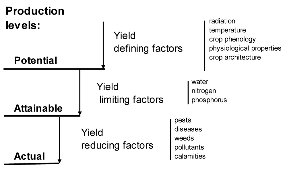
Figure 8.1. Relationships among potential, attainable and actual yields and growth-defining, growth-limiting and growth-reducing factors (Rabbinge, 1993; van Ittersum and Rabbinge, 1997).
The
potential yield (Yp) of a crop is determined by
defining factors: radiation, temperature, and morphological and physiological attributes determined by the genotype of the crop. The potential yield thus corresponds to the yield that would be produced by a crop grown under optimum conditions.
The
attainable yield (Ya) is determined by the defining factors in combination with
limiting factors: water and nutrients. The attainable yield corresponds also to the yield that would be produced by a crop when free of
injuries.
The combination of yield defining and yield limiting factors can be embedded in the concept of
production situation (de Wit and Penning de Vries, 1982; Savary and Zadoks, 1992; Rabbinge
et al., 1993).
The attainable yield of a given crop thus corresponds to the production situation under which this crop is grown.
The attainable yield can be reduced by the effect of
reducing factors such as
pest (disease, insects, weeds)
injuries. An
injury is a visible, measurable symptom caused by a harmful organism (Zadoks, 1985).
The resulting yield, obtained in a crop that has been injured by one or several pests, is defined as the
actual yield,
Y (Rabbinge, 1993): the actual yield, therefore, is the crop yield actually harvested in a farmer’s field.
Yield loss (YL), or
damage (Zadoks,1985), represents the difference between the attainable and the actual yield; that is, the yield lost from pests’ injuries. Yield loss can be associated to individual pests as well as to multiple pests. The functional relationships between production situation, attainable and actual yields, yield losses and injuries are summarized in Fig. 8.2.
Yield loss is frequently expressed as the fraction (percentage) of the attainable yield lost to pest injuries. It is then called
relative yield loss (RYL), and is computed as:
RYL = 100 × [(Ya –
Y) /
Ya].
The relationship between injury levels and the yield loss they cause is one important quantitative component analyzed when addressing yield losses. This relationship is called a
damage function.
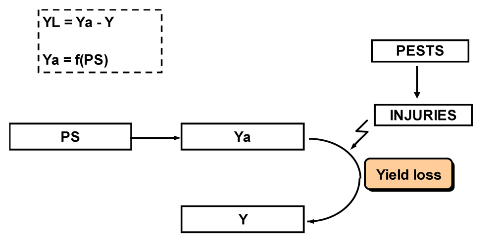
Figure 8.2. Relationships between production situation (PS), attainable yield (Ya), and actual yield (Y); yield loss (YL) (Willocquet et al., 1998).
Production situations may correspond to varying levels of attainable and actual yields, as illustrated in Fig. 8.3. For example:
- two different production situations (i.e., combinations of yield-defining and yield-limiting factors) may correspond to the same level of
Ya, but to different levels of yield losses (i.e., different combinations of pest injuries), and therefore to different actual yields (PS1 and PS2);
- two production situations may correspond to different levels of
Ya, but to the same level of actual yield (because yield losses are different: PS2 and PS3);
- two production situations may correspond to different levels of
Ya and actual yield (PS3 and PS4), the ranking of yield levels between the two production situations being the same (YaPS3>YaPS4 and YPS3 > YPS4);
- two production situations may correspond to different levels of
Ya and actual yield (PS4 and PS5), the ranking of yield levels between the two production situations being opposite (YaPS4 > YaPS5 and YPS4 < YPS5).
This diversity of possibilities implies that the quantification of the relative role of the different factors determining the actual yield is a first step when aiming at improving agrosystems' performance.
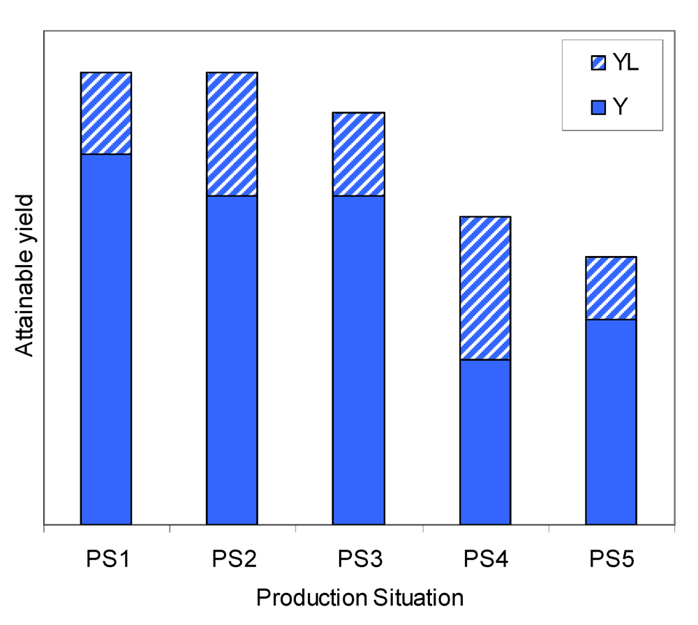
Figure 8.3. An illustration of yield levels in a range of production situations.The concept of damage mechanisms
Damage functions, which quantify the relationships between injuries and yield losses (Zadoks, 1985), can be determined experimentally. They can also be determined from crop loss simulation models, because, as processes, the damage functions represent processes that are underpinned by sub-processes:
damage mechanisms (DM). In these models, the processes involved in plant growth are represented, as well as DMs. Damage mechanisms refer to the processes involved in crop growth that are affected by a harmful agent. Different mechanisms can be described (Rabbinge and Rijsdijk, 1981; Boote et al., 1983). The main categories of DMs are listed in Table 8.1.
Table 8.1. Damage mechanisms of crop pest injuriesa
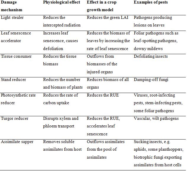
aDerived from Rabbinge and Vereyken (1980), Rabbinge and Rijsdijk (1981) and Boote et al. (1983).
Damage mechanisms have been experimentally measured for many pests, for example on groundnut rust (Savary et al., 1990), rice leaf blast (Bastiaans, 1991), bean diseases (Bassanezi et al., 2001; Lopes et al., 2001), and wheat
Septoria tritici blotch (Robert et al., 2006). Such quantification allows a better understanding of the underlying mechanisms of the effects of pests on crop growth.
The use of DM parameters can serve at least three purposes:
- DMs can be incorporated into models simulating components of crop growth, e.g., canopy photosynthesis (Bastiaans and Kropff, 1993), and assimilate partitioning (Bancal et al., 2012).
- DMs can be incorporated in crop growth simulation models in order to simulate their effect of crop growth and yield. How to implement this will be described in section 8.4, and examples from the literature are given in the introduction of this chapter.
- parameters for DMs can also be used to compare host plant resistance levels amongst genotypes of a given crop (e.g., Bastiaans and Roumen, 1993).
The use of damage mechanism parameters illustrates again one important characteristic of mechanistic simulation modeling, that is, the mobilization of parameters that have been acquired
experimentally. Therefore, there is no disconnection, but, to the contrary,
a complete loop from experimental data to model (parameters)
and from model to experiments (experimentally measured system's response).
The effects of pests on crop growth using the RI-RUE framework
The damage mechanisms described above can be linked to the RI-RUE concepts described in the previous chapter. Johnson (1987) grouped damage mechanisms in two broad categories, according to their major effect on RI (the first four damage mechanisms: light stealers, leaf senescence accelerators, tissue consumers, and stand reducers) and RUE (the last three damage mechanisms: photosynthetic rate reducer, turgor reducers, and assimilate sappers).
Using a potato crop growth simulation model including damage mechanisms for several pests, Johnson (1987) exemplified the effects of injuries on yield losses according to their yield-reducing effects (through a reduction of RI or of RUE; Fig. 8.4).

Figure 8.4. Types of damage functions corresponding to RI-reducing and RUE-reducing pests (derived from Johnson, 1987).
Because of Beer's law relationship between LAI and RI, a pest reducing the LAI will have a small reducing effect on yield at low pest intensity. On the other hand, RUE-reducing pests will have a large effect even at low pest intensity, and this effect will decrease (relatively) as pest intensity (and injury) increases.
Grouping pests according to their effects on RI and RUE may be useful for crop loss assessment and disease (pest) management. Analyzing these relationships (damage function, damage mechanism, RI-RUE-reducing effect) allows one to:
(1) address this type of research question in a synthetic way, while
(2) still accounting for the underlying biological mechanisms.
These underlying mechanisms involve questions pertaining to (1) the impact of pests on yield losses, (2) the injury thresholds for pest management, and (3) multiple-pest systems (Johnson, 1987). This approach has been used to analyze many, diverse, pathosystems. It remains very appealing when analyzing interactions between pests, yield, and production situations (Savary et al., 2006). The simplicity of the framework may provide an appealing way for analyses incorporating other factors, e.g., decision making or incorporating other species such as antagonists.
A simple crop growth simulation model for actual growth and yield, and yield losses – GENEPEST
Stages to simulate yield losses, and possible outcomes
Simulation of crop growth and yield affected by pest injuries can be made by incorporating into a crop growth model (such as GENECROP) the damage mechanisms corresponding to the injuries addressed. We shall call this new model GENEPEST. A complete listing of the program can be found in Appendix 8.1.
A three-stage approach then allows the simulation of yield losses:
1. Simulation of non-injured growth, enabling one to model the attainable growth and attainable yield (Ya) of a crop under a given production situation. By definition, all injury levels are then set to zero.
2. Simulation of growth under specified levels of injuries in order to model the actual growth and actual yield (Y).
3. Computation of yield losses, that is, the difference between simulated attainable and actual yields.
Note 1. Simulating growth and yield with levels of injuries corresponding to improved pest management (Ym) allows estimating yield that would be gained on the actual yield (Y) from this improvement in pest management (Ym-Y), thus providing a basis to guide strategic decisions such as research priorities in pest management.
Note 2. Yield losses can be simulated for a range of production situations, by setting the crop drivers (i.e., parameters and interpolation functions for crop growth) to values corresponding to each production situation, and proceeding to the three stages described above.
Note 3. Yield losses can be simulated for injuries considered individually and for combinations of injuries (i.e., grouped as pre-defined injury profiles), thus allowing ranking injuries according to their importance in terms of the yield losses they cause. Such results can help in ranking crop health problems and, again, help for guiding research priorities in pest management.
Incorporating damage mechanisms into a crop growth model
The damage mechanisms given in Table 8.1 can be incorporated in the crop growth model, GENECROP described in the previous chapter, leading to the GENEPEST model (Fig. 8.5).
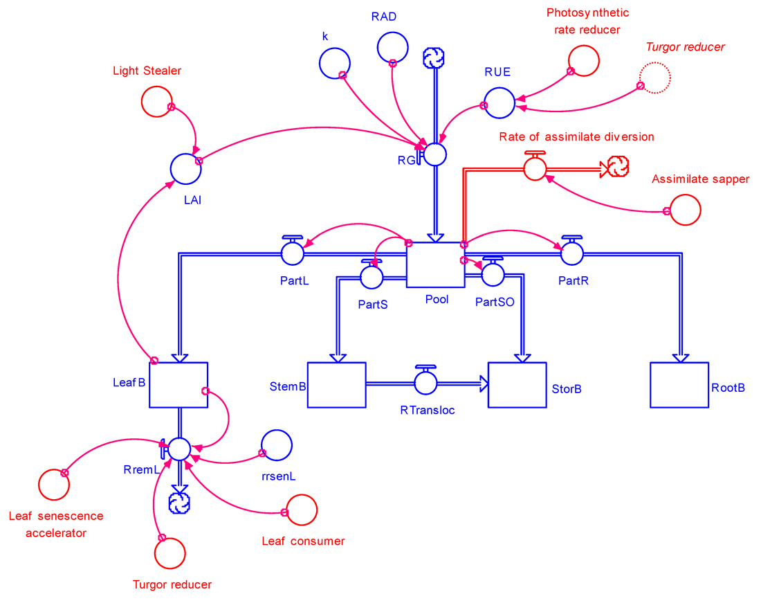
Figure 8.5. GENEPEST: general structure of a crop growth model incorporating damage mechanisms from pest injuries.
Stand reducers are not included in Fig 8.5 in order to avoid crowding the diagram. Stand
reducers would affect the biomass of all organs, and would be reflected by rates of reduction of biomass for all for organs.
Fig. 8.5 indicates that:
all damage mechanisms can be accounted for in GENEPEST,
the different damage mechanisms correspond in general to effects on different processes (rates) or on different variables,
different damage mechanisms however can affect the same process (i.e., leaf consumers and leaf senescence accelerators cause a reduction in [green] leaf biomass, and
a damage mechanism can affect more than one process or variable, as in the case of turgor reducers.
Damage mechanisms are now considered with examples from varying pests in order to illustrate how damage mechanisms can be coupled to a crop growth model.
Light stealers
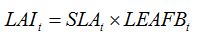
Light stealers decrease the area of green LAI. This typically corresponds to leaf diseases. Thus, equation (7.6) in Chapter 7:
|
 | (7.6) |
becomes, for one leaf disease, LD1:
 | (8.1) |
where
RF stands for the 'Reduction Factor' associated to the injury caused by leaf disease 1.
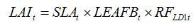
Note that this reduction factor is dynamic, as indicated by the
t index. In the case of a foliar disease, which produces lesions that decrease the green LAI, equation (8.1) can be simply written as:
 | (8.2) |
where
xLD1t is the disease severity of LD1 (i.e., the fraction of leaves covered by lesions varying between 0 and 1) at time
t. Equation (8.1) reflects the decrease in (green) LAI caused by disease, which corresponds to the leaf area covered by lesions and not photosynthesizing any more. Again, the reduction in LAI is dynamic, as disease severity can be made to vary over the course of an epidemic.
If we consider three leaf diseases LD1, LD2, LD3, equation (8.2) becomes:
 | (8.3) |
The underlying hypotheses of this equation are that (1) decreases in LAI can be due to one disease only (overlapping of lesions from two different diseases will reduce the LAI only once), and (2) the three diseases are randomly distributed in the crop canopy.
Leaf senescence accelerators and tissue (leaf) consumers
Leaf senescence accelerators and leaf consumers generally refer to different pests, the former typically corresponding to pathogens, and the second to insect defoliators. From a modeling point of view, they are however handled together and in the same manner here, because they correspond to the same effect on crop growth, i.e., a reduction in leaf dry biomass. The incorporation of these effects into the model is first described in the case of leaf senescence accelerators and then in the case of leaf consumers.
Leaf senescence accelerators have the same physiological effect as physiological senescence, and are therefore accounted for in the crop growth model in the same way as physiological senescence. So, equation 7.18 in Chapter 7:
 | (7.18) |
becomes:
 | (8.4) |
where
RSENIN1
t is the rate of leaf senescence caused by injury. It is convenient to establish a relationship between
RSENIN1 and injury level by expressing this rate of senescence as the product of a relative rate of senescence by the leaf dry biomass:
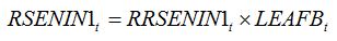 | (8.5) |
with:
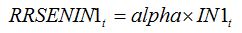 | (8.6) |
Equations (8.5) and (8.6) simply mean that in the case of leaf senescence caused by an injury, the fraction of leaf senesced is proportional to the intensity of the injury. Injury can be expressed as disease severity (i.e., a fraction between 0 and 1). The magnitude of the effect of injury on senescence corresponds to the parameter
alpha, which needs to be measured experimentally.
An important example of tissue consumers is the case of defoliating insects, which decrease the leaf biomass by eating leaves or fractions of leaves. This type of damage mechanism can be reflected in equation (7.18) by reducing the leaf biomass as a result of consumption by defoliating insects:
 | (8.7) |
where
RDEFt is the rate of defoliation. In the same way as for senescence accelerators, a relationship can be established between the rate of defoliation and the injury:
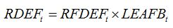 | (8.8) |
with
RFDEFt is the rate of increase in fraction of leaf area damaged by defoliation. This rate can be derived from successive assessments of the fraction of leaf area defoliated.
When combining effects of senescence accelerators and leaf consumers, the following hypothesis is made: leaf consumers do not damage leaf tissues that are senesced, and leaf senescence cannot occur on defoliated parts of leaves. The combined effects of these two damages are therefore additive and can be written as:
 | (8.9) |
Photosynthetic rate reducersPhotosynthetic rate reducers can be incorporated in a crop growth model such as GENECROP (chapter 7) by decreasing the RUE. In crop growth models describing in more detail the photosynthesis processes, the effect of photosynthetic rate reducers would be reflected by a reduction in, for example, the initial light use efficiency of single leaves, and/or a reduction in the maximum rate of photosynthesis, and/or an increase in dark respiration (e.g., Rossing et al., 1992).
In GENECROP, equation 7.5 in Chapter 7:
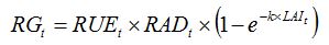 | (7.5) |
becomes:
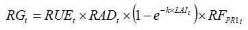 | (8.10) |
In the case of light stealers such as (leaf-spotting) foliar diseases, the relationship between the reduction factor and the level of injury is straightforward: the reduction in green LAI corresponds to disease severity and
RF =1 -
x = 1 - severity.
When addressing photosynthetic rate reducers, the relationship between the reduction factor and the level of injury is less straightforward, and often needs to be established experimentally. Two examples corresponding to pests which widely differ biologically (a viral disease and a root-infecting disease), but nevertheless cause similar damage mechanisms by reducing the
RUE, are given below to illustrate how
RF can be expressed.
Viral diseases are in general systemic and the virus particles are transported within the plant via its vascular system. Virus infection can reduce the rate of photosynthesis and this can be simply represented by the relationship between the proportion of disease plants and the reduction factor:
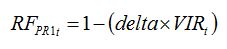 | (8.11) |
where
delta is a parameter ranging between 0 and 1, which represents the magnitude in the effect of viral infection to reduce the
RUE, and
VIRt is the proportion of diseased plants. The parameter
delta needs to be measured with specific experiments.
Root-infecting diseases cause injuries, which directly affect the functioning of infected roots, and therefore the amount of water and nutrients absorbed by the roots. This in turn causes a reduction in
RUE. A relationship between the disease level and
RF can be written as:
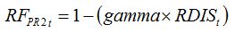 | (8.12) |
where, similarly to equation (8.11),
gamma is a parameter ranging between zero and 1, which represents the magnitude in the effect of root infection to reduce the
RUE, and
RDISt is the proportion of roots infected by the pathogen. The parameter
gamma needs to be measured with specific experiments.
Accounting for the combined effects of the two above pests can be done by multiplying the reduction factors, which reflects (1) the interactions between both pests in their effect on RUE and (2) the hypothesis of random distribution of both pests. Equation (8.10 becomes:
 | (8.13) |
Assimilate sappersAssimilate sappers uptake assimilates produced from photosynthesis. Two important pest groups cause this type of damage mechanism: insects such as aphids or plant hoppers which are feeding from the phloem sap, and biotrophic fungi such as rusts which are diverting the assimilates to produce fungal organs, especially spores. One could also add a number of plant nematodes, at least those which do not cause tissue necrosis.
The diversion of assimilates is accounted for in the simulation of the dynamics of the pool of assimilates. Equation (7.16) from Chapter 7:
 | (7.16) |
becomes:
 | (8.14) |
The amount of assimilates diverted by pests is retrieved from the amount of assimilates partitioned towards organs, and equations (7.12) to (7.15) in Chapter 7 become:
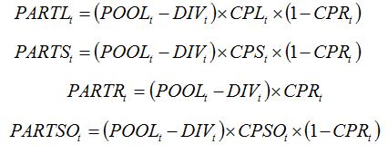 | (8.15)
(8.16)
(8.17)
(8.18) |
Again, a relationship needs to be established experimentally between the amount of assimilates diverted by the pest and the level of injury. In the case of insects, this corresponds to the sapping (or sucking) rate, and can depend on the crop development stage and the insect development stage (or weight). The diversion rate can be written as:
 | (8.19) |
where
DIVINSt is the (daily) assimilate diversion rate,
rrsapt is the relative rate of sapping (per biomass of insect and per day),
bmperinst is the biomass of an individual insect, and
NBINSt is the number of insects (per m
2),
rrspapt and
bmperinst need to be experimentally measured and may vary over time, and
NBINSt is the insect pest driving function, which may vary over time, and represents the dynamics of insect density.
In the case of biotrophic fungi, the relationships between disease intensity and the diversion of assimilates can be done according to the carbohydrate uptake for spore production, the number of spores produced per lesion per day, and the lesion size:
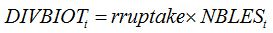 | (8.20) |
with:
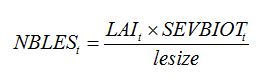 | (8.21) |
where
rruptake is the rate of carbohydrate uptake per lesion per day; and the number of lesions is derived from disease severity,
SEVBIOTt (pest driver), lesion area (lesize), and LAI.
When combining the two above pests, a simple hypothesis corresponds to the independence between both pests and their injuries, leading equation (8.14) to become:
 | (8.22) |
and replacing
POOLt -
DIVt by
POOLt -
DIVINSt -
DIVBIOTt in equations (8.15) to (8.18).
Turgor reducer
Damage mechanisms associated with turgor reducers have been addressed when considering RUE reducers and leaf senescence accelerators. They will therefore not be illustrated specifically in this chapter. Accounting for turgor reducers will however be illustrated in the next chapter.
Important note: for the sake of simplicity, the incorporation of damage mechanisms into a crop growth simulation model has been described above for each damage mechanism, one at a time.
Individual crop pests can, however, cause more than one type of damage. This will be illustrated in the GENEPEST model, and in the description of RICEPEST and WHEATPEST models in the next chapter.
Model parameters for damage mechanisms
The parameters needed to simulate damage mechanisms are derived from experiments. Two main types of parameters can be considered:
parameters which represent the magnitude of the impact of pest injuries on the crop physiological processes:
alpha (leaf senescence accelerator);
delta (virus disease – effect on RUE);
gamma (root-infecting disease – effect on RUE);
rrsap (insect sapper – rate of sapping); and
rruptake (biotrophic pathogen – rate of assimilate uptake).
parameters corresponding to ecological characteristics of the pests, which are needed to determine a relationship between the damage mechanism and the level of injury:
The following values are set in GENEPEST (again, these have to be experimentally measured for a given pest).
alpha = 0.076 day-1 (case of rice sheath blight; Willocquet et al., 2000)
delta = 0.35 (case of wheat BYDV; Willocquet et al., 2008)
gamma = 1 (case of wheat take-all; Willocquet et al., 2008)
rrsap = 1 mg·mg-1· day-1 (arbitrarily chosen value)
rruptake = 4.62 × 10⁻⁶ day-1 (case of wheat brown or leaf rust; Willocquet et al., 2008)
bmperins = 0.5 mg (arbitrarily chosen value)
lesize = 10-6 m2 (case of wheat brown or leaf rust; Willocquet et al., 2008)
Model drivers for pests injuries
The damage mechanisms described above have been implemented into GENEPEST by considering several pests, which provide a combination of the damage mechanisms described previously. The pests considered are described in Table 8.2.
Table 8.2. Examples of pests accounted for in GENEPESTa

aWeeds can also accounted for in a simplified manner, see
Chapter 9.
Simulations
The STELLA model GENEPEST.STMX will allow you to:
- explore the model structure and equations,
- explore the model inputs, especially the driving functions of the different pests included
- explore the model outputs, and
- run the model with varying levels of injury, which will allow you to explore:
- the effects of individual injuries on crop growth and yield
- the effects of combined injuries on crop growth and yield
Summary
This chapter describes:
- Concepts and definitions related to yield levels, production situations and injuries
- The concept of damage mechanism
- The effects of pests on crop growth within the RI-RUE framework
- How damage mechanisms are captured in a quantitative and dynamic way into a generic simulation model, GENEPEST.
- Provides the equations, parameters, and flowchart of GENEPEST.
- Includes the STELLA file, which can be used to explore the model structure and the effect of injuries, individually or in combination, on the simulated dynamics of crop growth.
References
Bancal, M. O., Hansart, A., Sache, I., and Bancal, P. 2012. Modelling fungal sink competitiveness with grains for assimilates in wheat infected by a biotrophic pathogen. Ann. Bot. 110:113-123.
Bassanezi, R. B., Amorim, L., Bergamin Filho, A., Hau, B., and Berger, R. D. 2001. Accounting for photosynthetic efficiency of bean leaves with rust, angular leaf spot and anthracnose to assess crop damage. Plant Pathol. 50:443-452.
Bastiaans, L. 1991. Ratio between virtual and visual lesion size as a measure to describe reduction in leaf photosynthesis of rice due to blast. Phytopathology 81:611-615.
Bastiaans, L. 1993. Effects of leaf blast on growth and production of a rice crop. 2. Analysis of the reduction in dry matter production, using two models with different complexity. Neth. J. Plant Pathol. 99 (suppl3):19-28.
Bastiaans, L., and Kropff, M. J. 1993. Effects of leaf blast on photosynthesis of rice. 2. Canopy photosynthesis. Neth. J. Plant Pathol. 99:205-217.
Bastiaans, L., and Roumen, E. C. 1993. Effect on leaf photosynthetic rate by leaf blast for rice cultivars with different types and levels of resistance. Euphytica 66:81-87.
Boote, K. J., Jones, J. W., Mishoe, J. W., and Berger, R. D. 1983. Coupling pests to crop growth simulators to predict yield reductions. Phytopathology 73:1581-1587.
Chiarappa, L. 1971. Crop Loss Assessment Methods: FAO Manual on the Evaluation and Prevention of Losses by Pests, Diseases and Weeds. FAO - Commonwealth Agricultural Bureau, Farnham Royal, UK.
Johnson, K. B. 1987. Defoliation, disease, and growth: a reply. Phytopathology 77:1495-1497.
Johnson, K. B. 1992. Evaluation of a mechanistic model that describes potato crop losses caused by multiple pests. Phytopathology 82:363-369.
Loomis, R. S., and Adams, S. S. 1983. Integrative analyses of host-pathogen relations. Annu. Rev. Phytopathol. 21:341-362.
Lopes, D. B., and Berger, R. D. 2001. The effects of rust and anthracnose on the photosynthesis competence of diseased bean leaves. Phytopathology 91:212-220.
Madden, L. V., Hughes, G., and Irwin, M. E. 2000. Coupling disease-progress-curve and time-of-infection functions for predicting yield loss of crops. Phytopathology 90:788-800.
Rabbinge, R. 1993. The ecological background of food production. Pages 2-29 in: Crop Protection and Sustainable Agriculture. Ciba Foundation 77. D. J. Chadwick and J. Marsh, eds. John Wiley & Sons, Chichester, UK.
Rabbinge, R., Ward, S. A., and Van Laar, H. H., eds. 1989. Simulation and Systems Management in Crop Protection. Pudoc, Wageningen, The Netherlands.
Rabbinge, R., and Rijsdijk, P. H. 1981. Disease and crop physiology: a modeler’s point of view. Pages 201-220 in: Effects of Disease on the Physiology of the Growing Plants. P. G. Ayres, ed. Cambridge Univ. Press, Cambridge, UK.
Rabbinge, R., and Vereyken, P. H. 1980. The effects of diseases or pests upon host. Z. Pflanzenk. Pflanzensch. 87:409-422.
Robert C., Bancal, M. O., Lannou, C., and Ney, B. 2006. Quantification of the effects of
Septoria tritici blotch on wheat leaf gas exchange with respect to lesion age, leaf number, and leaf nitrogen status. J. Exp. Bot. 57:225-234.
Rossing, W. A. H., van Oijen, M., van der Werf, W., Bastiaans, L., and Rabbinge, R., 1992. Modelling the effects of foliar pests and pathogens on light interception, photosynthesis, growth rate and yield of field crops. Pages 161–180 in: Pests and Pathogens. Plant Responses to Foliar Attack. P. G. Ayres, ed. Bios Scientific, Oxford, UK.
Savary, S., De Jong, P. D., Rabbinge, R., and Zadoks, J. C. 1990. Dynamic simulation of groundnut rust: a preliminary model. Agric. Syst. 32:113-141.
Savary, S., and Zadoks, J. C. 1992. An analysis of crop loss in the multiple pathosystem groundnut - rust - late leaf spot. II . A study of the interactions between diseases and crop intensification in factorial experiments. Crop Prot. 11:110-120.
Savary, S., Teng, P. S., Willocquet, L., and Nutter, F. W., Jr. 2006. Quantification and modeling of crop losses: a review of purposes. Annu. Rev. Phytopathol. 44:89-112.
Teng, P. S., ed. 1987. Crop Loss Assessment and Pest Management. APS Press, St Paul MN.
Van Ittersum, M. K., and Rabbinge, R. 1997. Ecology for analysis and quantification of agricultural input-output combinations. Field Crops Res. 52:197-208.
Willocquet, L., Savary, S., Fernandez, L., Elazegui, F. A., and Teng, P. S. 1998. Simulation of yield losses caused by rice diseases, insects, and weeds in tropical Asia. IRRI Discussion Paper Series no 34. IRRI, Los Baños, Philippines.
Willocquet, L., Savary, S., Fernandez, L., Elazegui, F. A., and Teng, P. S. 2000. Development and evaluation of a multiple-pest, production situation specific, simulation model of rice yield losses in tropical Asia. Ecol. Model. 131:133-159.
Willocquet, L., Aubertot, J. N., Lebard, S., Robert, C., Lannou, C., and Savary, S. 2008. Simulating multiple pest damage in varying winter wheat production situations. Field Crops Res. 107:12-28.
Wit, C. T. de, and Penning de Vries, F. W. T. 1982. L'analyse des systèmes de production primaire. Pages 20-27 in: La Prodctivité de Pâturages Sahéliens. F. W. T. Penning de Vries and M. A. Djiteye, eds. Agricultural Research Reports 918. Pudoc, Wageningen.
Zadoks, J. C. 1985. On the conceptual basis of crop loss assessment: the threshold theory. Annu. Rev. Phytopathol. 23:455-473.
Zadoks, J. C., and Schein, R. D. 1979. Epidemiology and Plant Disease Management. Oxford University Press, New York, USA.
Exercises and questions
1. Give examples of pests in wheat categorized by damage mechanism, following Table 8.1.
2. Indicate which of the following statement is (are) correct
- yield loss is the difference between attainable and actual yield
- yield loss is the difference between potential and attainable yield
- a yield reducing factor may be associated to different injury mechanisms
- a given damage mechanism can affect different physiological processes
3. A light stealer affects
- the RUE
- the partitioning towards organs
- the leaf biomass
- the LAI
4. Acceleration of leaf senescence affects
- the RUE
- the partitioning towards organs
- the leaf biomass
- the LAI
5. A possible unit for the relative rate of leaf senescence is
- g·g-1·day-1
- g·day-1
- g·g-1
- g·m-2·day-1
Answers to exercises and questions
1. pests by damage mechanism in wheat:
b. light stealer: weeds, Septoria blotch;
c. leaf senescence accelerator: Septoria blotch;
d. tissue consumer: many defoliating insects (e.g., Lema spp.);
e. stand reducer: many soil pathogens: take-all pathogen (e.g.,
Gaeumannomyces tritici); weeds; barley yellow dwarf virus disease;
f. photosynthetic rate reducer: barley yellow dwarf virus disease; Septoria blotch;
g. turgor reducer: eyespot pathogen (Rhizoctonia spp.);
h. Assimilate sappers: rust pathogens (stripe [yellow], leaf [brown], and stem rust); aphids.
2. a: yield loss is the difference between attainable and actual yield, and c: a yield reducing factor may be associated to different injury mechanisms
3. a: the LAI.
4. c: the leaf area biomass
5. a: g·g-1·day-1.
Appendix 8.1. Program listing of GENEPEST
LeafB(t) = LeafB(t - dt) + (PartL - RSenL) * dt
INIT LeafB = 10
INFLOWS:
PartL = CPL*(Pool-rdiv)
OUTFLOWS:
RSenL = ((rrsen+(alpha*LD2)+RFDEF)*LeafB)
MaxStemb(t) = MaxStemb(t - dt) + (rmaxstemb) * dt
INIT MaxStemb = 6
INFLOWS:
rmaxstemb = PartS
Pool(t) = Pool(t - dt) + (RGrowth - PartS - PartL - PartO - PartR - rdiv) * dt
INIT Pool = 0
INFLOWS:
RGrowth = RAD*RUE*(1-EXP(-k*LAI))*(1-(delta*VIR))*(1-(gamma*RDIS))
OUTFLOWS:
PartS = CPS*(Pool-rdiv)
PartL = CPL*(Pool-rdiv)
PartO = CPO*(Pool-rdiv)
PartR = CPR*(Pool-rdiv)
rdiv = (rsrsap*bmperins*INS)+(rruptake*LAI*LD3/lesize)
REPTIL(t) = REPTIL(t - dt) + (Rmat - Rmortr) * dt
INIT REPTIL = 0
INFLOWS:
Rmat = if DVS<0.8 or DVS>1 then 0 else if VTIL
OUTFLOWS:
Rmortr = rrmort*REPTIL
RootB(t) = RootB(t - dt) + (PartR) * dt
INIT RootB = 5
INFLOWS:
PartR = CPR*(Pool-rdiv)
StemB(t) = StemB(t - dt) + (PartS - RTransloc) * dt
INIT StemB = 6
INFLOWS:
PartS = CPS*(Pool-rdiv)
OUTFLOWS:
RTransloc = IF(DVS>1) then ddist else 0
STEMP(t) = STEMP(t - dt) + (Dtemp) * dt
INIT STEMP = 320
INFLOWS:
Dtemp = ((TMAX+TMIN)/2)-TBASE
StorB(t) = StorB(t - dt) + (PartO + RTransloc) * dt
INIT StorB = 0
INFLOWS:
PartO = CPO*(Pool-rdiv)
RTransloc = IF(DVS>1) then ddist else 0
VTIL(t) = VTIL(t - dt) + (Rtil - Rmat - Rmrtv) * dt
INIT VTIL = 250
INFLOWS:
Rtil = PartLS*STW*(1-(VTIL/maxtil))*DVE
OUTFLOWS:
Rmat = if DVS<0.8 or DVS>1 then 0 else if VTIL
Rmrtv = (rrmort*VTIL)
alpha = 0.076
bmperins = 0.0005
CPL = CPPL*(1-CPR)
CPO = CPPO*(1-CPR)
CPS = (1-CPL-CPO)*(1-CPR)
DACE = TIME+14
ddist = 0.005*MaxStemb
delta = 0.35
DVS = if stemp
FST = 0.05
gamma = 1
grain__yield = 0.85*StorB
INS = pINS*INSn
k = 0.6
LAI = LeafB*SLA*(1-LD1)*(1-LD2)*(1-LD3)
LD1 = pLD1*LD1n
LD2 = pLD2*LD2n
LD3 = pLD3*LD3n
lesize = 0.000001
maxtil = 900
PartLS = PartL+PartS
pINS = 0
pLD1 = 0
pLD2 = 0
pLD3 = 0
pRDIS = 0
pRFDEF = 0
pVIR = 0
RAD = 17
RDIS = pRDIS*RDISn
RFDEF = pRFDEF*RFDEFn
RRMAT = 0.3
rruptake = 0.00000462
rsrsap = 1
RUE = 1.2
STW = 20
TBASE = 8
TFLOW = 1500
TMAT = 2000
TMAX = 30
TMIN = 24
Totil = VTIL+REPTIL
VIR = pVIR*VIRn
CPPL = GRAPH(DVS)
(0.00, 0.55), (0.1, 0.536), (0.2, 0.521), (0.3, 0.507), (0.4, 0.493), (0.5, 0.479), (0.6, 0.464), (0.7, 0.45), (0.8, 0.3), (0.9, 0.15), (1, 0.00), (1.10, 0.00), (1.20, 0.00), (1.30, 0.00), (1.40, 0.00), (1.50, 0.00), (1.60, 0.00), (1.70, 0.00), (1.80, 0.00), (1.90, 0.00), (2.00, 0.00)
CPPO = GRAPH(DVS)
(0.00, 0.00), (0.05, 0.00), (0.1, 0.00), (0.15, 0.00), (0.2, 0.00), (0.25, 0.00), (0.3, 0.00), (0.35, 0.00), (0.4, 0.00), (0.45, 0.00), (0.5, 0.00), (0.55, 0.00), (0.6, 0.00), (0.65, 0.00), (0.7, 0.00), (0.75, 0.00), (0.8, 0.143), (0.85, 0.286), (0.9, 0.429), (0.95, 0.571), (1.00, 0.714), (1.05, 0.857), (1.10, 1.00), (1.15, 1.00), (1.20, 1.00), (1.25, 1.00), (1.30, 1.00), (1.35, 1.00), (1.40, 1.00), (1.45, 1.00), (1.50, 1.00), (1.55, 1.00), (1.60, 1.00), (1.65, 1.00), (1.70, 1.00), (1.75, 1.00), (1.80, 1.00), (1.85, 1.00), (1.90, 1.00), (1.95, 1.00), (2.00, 1.00)
CPR = GRAPH(DVS)
(0.00, 0.3), (0.1, 0.263), (0.2, 0.225), (0.3, 0.188), (0.4, 0.15), (0.5, 0.112), (0.6, 0.075), (0.7, 0.038), (0.8, 0.00), (0.9, 0.00), (1, 0.00), (1.10, 0.00), (1.20, 0.00), (1.30, 0.00), (1.40, 0.00), (1.50, 0.00), (1.60, 0.00), (1.70, 0.00), (1.80, 0.00), (1.90, 0.00), (2.00, 0.00)
DVE = GRAPH(DVS)
(0.00, 1.00), (0.4, 1.00), (0.8, 0.00), (1.20, 0.00), (1.60, 0.00), (2.00, 0.00)
INSn = GRAPH(TIME)
(0.00, 0.00), (10.0, 0.00), (20.0, 0.00), (30.0, 50.0), (40.0, 100), (50.0, 150), (60.0, 200), (70.0, 150), (80.0, 100), (90.0, 50.0), (100, 5.00), (110, 5.00), (120, 5.00)
LD1n = GRAPH(TIME)
(0.00, 0.00), (10.0, 0.00), (20.0, 0.00), (30.0, 0.004), (40.0, 0.008), (50.0, 0.01), (60.0, 0.007), (70.0, 0.002), (80.0, 0.00), (90.0, 0.00), (100, 0.00), (110, 0.00), (120, 0.00)
LD2n = GRAPH(TIME)
(0.00, 0.00), (10.0, 0.00), (20.0, 0.00), (30.0, 0.002), (40.0, 0.005), (50.0, 0.008), (60.0, 0.01), (70.0, 0.008), (80.0, 0.007), (90.0, 0.006), (100, 0.005), (110, 0.004), (120, 0.004)
LD3n = GRAPH(TIME)
(0.00, 0.00), (10.0, 0.00), (20.0, 0.00), (30.0, 0.003), (40.0, 0.005), (50.0, 0.007), (60.0, 0.009), (70.0, 0.01), (80.0, 0.01), (90.0, 0.009), (100, 0.007), (110, 0.005), (120, 0.001)
RDISn = GRAPH(TIME)
(0.00, 0.00), (10.0, 0.00), (20.0, 0.00), (30.0, 0.001), (40.0, 0.002), (50.0, 0.01), (60.0, 0.01), (70.0, 0.01), (80.0, 0.01), (90.0, 0.01), (100, 0.01), (110, 0.01), (120, 0.01)
RFDEFn = GRAPH(TIME)
(0.00, 0.00), (10.0, 0.00), (20.0, 0.00), (30.0, 0.00), (40.0, 0.001), (50.0, 0.00), (60.0, 0.00), (70.0, 0.00), (80.0, 0.00), (90.0, 0.00), (100, 0.00), (110, 0.00), (120, 0.00)
rrmort = GRAPH(DVS)
(0.00, 0.00), (0.1, 0.00), (0.2, 0.00), (0.3, 0.00), (0.4, 0.00), (0.5, 0.02), (0.6, 0.02), (0.7, 0.02), (0.8, 0.02), (0.9, 0.02), (1, 0.00), (1.10, 0.00), (1.20, 0.00), (1.30, 0.00), (1.40, 0.00), (1.50, 0.00), (1.60, 0.00), (1.70, 0.00), (1.80, 0.00), (1.90, 0.00), (2.00, 0.00)
rrsen = GRAPH(DVS)
(0.00, 0.00), (0.1, 0.00), (0.2, 0.00), (0.3, 0.00), (0.4, 0.00), (0.5, 0.00), (0.6, 0.00), (0.7, 0.00), (0.8, 0.00), (0.9, 0.00), (1, 0.00), (1.10, 0.013), (1.20, 0.026), (1.30, 0.04), (1.40, 0.04), (1.50, 0.04), (1.60, 0.04), (1.70, 0.04), (1.80, 0.04), (1.90, 0.04), (2.00, 0.04)
SLA = GRAPH(DVS)
(0.00, 0.037), (1.00, 0.018), (2.00, 0.017)
VIRn = GRAPH(TIME)
(0.00, 0.00), (10.0, 0.00), (20.0, 0.00), (30.0, 0.002), (40.0, 0.01), (50.0, 0.01), (60.0, 0.01), (70.0, 0.01), (80.0, 0.01), (90.0, 0.01), (100, 0.01), (110, 0.01), (120, 0.01)

